Directivity
The Directivity plot () is an extension of the far-field plots and is a common acoustic plot for speakers, for example. The plot collects spatial information across frequencies and shows this information in a contour plot.
You can add Directivity plot nodes to 2D plot groups from the More Plots submenu.
Go to Common Results Node Settings for links to information about these sections: Data, Title, Levels, Range, Inherit Style, and Coloring and Style.
Expression
For the standard settings, see Expressions and Predefined Quantities. You can also choose a normalization of the data from the Normalization list:
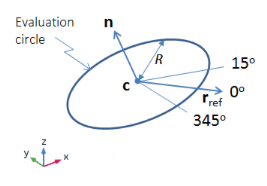
Choose With respect to angle (the default) to compute an expression with the level normalized with respect to the value at a specific angle. You specify the angle (in degrees) in the Angle field (unit: deg).
Choose With respect to maximum to compute the expression normalized with respect to its maximum level value for each frequency.
Choose None to not use any normalization.
Evaluation
Under Angles, enter the Number of angles. The default is 50.
Select a Restriction: None (the default) or Manual.
If Manual is selected, enter values (SI unit: deg) for:
start (the default is 0 degrees).
range (the default is 360 degrees). Typically the range will be 180 degrees to evaluate the directivity in the half space in front of a speaker.
Under Center, enter values for the coordinates at the center of the evaluation circle. Under Normal, enter the coordinates of the normal defining the evaluation plane. Under Evaluation distance, enter a Radius for the evaluation; the default is 1 m as usually used for these plots. Under Reference direction, specify the coordinates of the vector that specifics the direction representing 0 degrees in the plot. The entered vector is projected onto the evaluation plane. A schematic of the evaluation circle is given in Figure 20-3 below.
Figure 20-3: Schematic of the evaluation circle used in the Directivity and Far Field plots, showing the circle center c, evaluation plane normal n, evaluation radius R, and reference direction rref.
In 3D models, you can preview the evaluation plane, including circle, normal, and reference direction, in the geometry by clicking the Preview Evaluation Plane button at the bottom of the Evaluation section. An example of the resulting plot is depicted in Figure 20-4 below.
Figure 20-4: Preview plot of the evaluation circle used in the directivity plot for the Vented Loudspeaker Enclosure model from the Acoustics Module Application Gallery.
Coloring and Style
In addition to common coloring and style settings, you can specify the axis for the frequency. From the Layout list, choose:
Frequency on x-axis to plot with the frequency on the x-axis.
Frequency on y-axis to plot with the frequency on the y-axis.