Evaluating and plotting the acoustic pressure around radiating objects and sources is essential for the development of several acoustic devices. This is known as the spatial response. Application areas range from underwater acoustic transducers and loudspeakers, to determining the spatial sensitivity of microphone systems (for example, using reciprocity). Using the Far-Field Calculation feature can help to reduce the computational domain while still being able to determine the pressure and thus the spatial response in the near-field to far-field. The Far Field plots are specially designed for easy evaluation of the far-field variables, that is, the acoustics far-field pressure and the far-field sound pressure level.

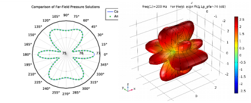
In the Far Field plots the far-field variable (pressure or sound pressure level) is represented in a polar plot for a selected number of angles. Data is retrieved on an evaluation circle in 2D, 2D axial symmetry, or 3D. The angle interval and the number of angles can be manually specified. The evaluation circle origin, orientation, and radius can be specified as well as the reference direction. The evaluation circle can be visualized using a Preview Evaluation Plane functionality. There is also a built in option to calculate the Beam Width of the plotted data. A 3D polar plot also exists where the data is evaluated on a sphere. For 3D far-field plots you also specify an expression for the surface color.

Another way of evaluating and depicting the far field is by using either the Grid 2D, the Grid 3D, the Parametrized Curve, or the Parametrized Surface data sets. Both types of data sets allow the evaluation of global quantities, like the far-field variables, outside of the computational domain (outside of the mesh).

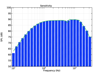
A dedicated Octave Band () plot exists to plot frequency response, transfer functions, transmission loss, and insertion loss curves. The plot has several built in acoustics specific features like predefined weighting (Z, A, C, and user defined) as well as the possibility to plot the response in octaves, 1/3 octaves, or as a continuous response.

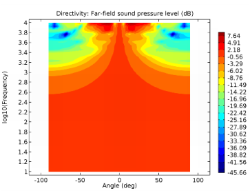
Another acoustics specific plot, especially used for loudspeakers, is the dedicated Directivity () plot. The plot allows audio engineers to depict the spatial response of a loudspeaker as function of both frequency and spatial angle in a contour like plot. Representing the spatial response in this manner is a very common the loudspeaker industry. Measured data is often also represented in the same manner. The plot includes many options to format the plot to achieve maximal insight into the modeled data, for example, easy switch of the x- and y-axis (frequency and polar angle axis) as well as options to normalize the data with respect to a given angle or the maximal value.