COMSOL 6.4 - Setting Up a Contact Problem

Setting Up a Contact Problem

Mechanical contact can be modeled between boundaries in the Solid Mechanics; Solid Mechanics, Explicit Dynamics; Multibody Dynamics; Shell; Layered Shell; and Membrane interfaces. You can model contact not only within a single physics interface, but also between two physics interfaces, or even between a physics interface and any boundary having a mesh, using a combination of and nodes.


	The General Contact node is available in the Solid Mechanics; Solid Mechanics, Explicit Dynamics; and Multibody Dynamics interfaces.

Within the Solid Mechanics and Solid Mechanics, Explicit Dynamics interfaces, you can either use the more general formulations available through the and nodes, or you can use a simplified version called .

Using Contact Pairs and the Contact Node

To model a mechanical contact problem using the node, you must do the following fundamental steps:

•

In the finalization step of the geometry sequence, you should normally have set to . If is used, then the contacting boundaries must be geometrically separated in the initial configuration.

•

Add a (

) under . A contact pair defines a mapping between two sets of boundaries; the source and destination boundaries. Contact pairs can also be added automatically, based on boundary adjacency when the action is used.

•

Use the default node or add new nodes in the physics interface. In the node, you select the contact pairs to be used, and provide the settings for the physical and numerical properties of the contact model.

•

If relevant, add , , , , or subnodes to .

•

Select a suitable study type. You can analyze contact using the following types of study steps:

Stationary; commonly using an auxiliary sweep.

Bolt Pretension

Time Dependent

Explicit Dynamics

Any type of prestressed analysis. In this case, the full contact problem is solved in the preload step, and in the subsequent perturbation step the contact state is considered as fixed.

The fact that you add a node to your model will automatically make all study steps geometrically nonlinear. For the default node, this requirement can be removed by selecting .


	Because of the multiphysics capabilities of COMSOL Multiphysics, the setup of a contact problem is split into two parts. The definition of the contact pair is made under Definitions, and can be shared between several physics interfaces. This part of the contact problem defines the geometric properties of the contact, such as search and mapping operations between the selected boundaries. The physics-related definitions are then made in the respective physics interfaces.

When to Use the Contact Pair Formulation

The contact pair provides a general formulation that can handle arbitrarily large deformations including finite sliding with or without friction. For cases where you know which boundaries may interact through contact when setting up the model, it is often the preferred option. It limits the size of the contact problem to selected boundaries, thus keeping down the computational cost and complexity.

The node includes a wide range of contact methods ranging from the lean and robust but approximate penalty method, to the more accurate but expensive augmented Lagrangian and Nitsche methods. The latter methods are not supported by . Thus, for contact interactions where high accuracy is important, use the node.

Complex contact interactions involving , , and can only be modeled using the node.

In a multiphysics analysis, the contact pair formulation can also incorporate for example changes in the heat flux or electric current through the contacting boundaries. You will then also need to add corresponding features in the other participating interfaces, like a node in the Heat Transfer in Solids interface. The contact state and contact pressure used by other physics interfaces are always supplied by the structural mechanics interface

•

Documentation of the Contact, Friction, Slip Velocity, Adhesion, Decohesion, and Wear nodes.

•

Contact Analysis Theory.

•

Identity, Contact, and Sector Symmetry Pairs in the COMSOL Multiphysics Reference Manual.

Using General Contact Pairs and the General Contact Node

To model a mechanical contact problem using the node, you must do the following fundamental steps:

•

Add a (

) under . By default, a general contact pair defines a mapping between all geometric objects in the model, including domains and free boundaries. When all objects are included, a single general contact pair is sufficient.

•

Use the default node or add new nodes in the physics interface. In the node, you select the general contact pairs to be used.

•

The main settings for the physical and numerical properties of the contact model are made in the subnode. Add more nodes to use different settings for different boundaries. Geometric properties of boundaries can be adjusted by adding subnodes.

•

If relevant, add or subnodes to .

•

Select a suitable study type. You can analyze contact using the following types of study steps:

Stationary; commonly using an auxiliary sweep.

Bolt Pretension

Time Dependent

Explicit Dynamics

Any type of prestressed analysis. In this case, the full contact problem is solved in the preload step, and in the subsequent perturbation step the contact state is considered as fixed.

The fact that you add a node to your model will automatically make all study steps geometrically nonlinear. For the default node, this effect can be removed by selecting .

When to Use the General Contact Pair Formulation

The general contact pair provides a general formulation that can handle arbitrarily large deformations including finite sliding with or without friction. Compared to the contact pair formulation, contact detection is automatic with no need to distinguish between source and destination boundaries, making it easy to set up the contact problem even for large and complex assemblies. Special contact situations, such as self-contact, are also intrinsically supported with no extra modeling steps required.

A typical usage of the general contact pair is to let it define the overall contact interaction for the entire geometry, while other pairs define interactions for specific boundaries where more detail is required. For example, add a contact pair to use the more accurate augmented Lagrangian method in a bolted connection, or add an identity pair to model continuity between a set of boundaries.

•

Documentation of the General Contact, Contact Model, Offset, Damping (General Contact), and Friction (General Contact)nodes.

•

Contact Analysis Theory.

•

Identity, Contact, and Sector Symmetry Pairs in the COMSOL Multiphysics Reference Manual.

Using the Interior Contact node

To model a mechanical contact problem using the node, you must do the following fundamental steps:

•

Add an node.

•

Select the set of boundaries that form the region where contact is defined.

•

Provide the settings for the physical and numerical properties of the contact model.

•

If relevant, add , , or subnodes.

•

Select a suitable study type. You can analyze contact using the following types of study steps:

Stationary; commonly using an auxiliary sweep.

Bolt Pretension

Time Dependent

Explicit Dynamics

Any type of prestressed analysis. In this case, the full contact problem is solved in the preload step, and in the subsequent perturbation step the contact state is considered as fixed.

When to Use the Interior Contact Formulation

The interior contact formulation does not require the addition of any contact pairs. It is applied as a slit condition on an interior boundary in a solid. A slit condition keeps the mesh, but allows different displacements on the elements on the two sides of the boundary. The computationally expensive contact search is avoided, instead the gap and sliding distances are measured as the difference in displacements across the slit. This also has the advantage that does not force a geometrically nonlinear study.

The interior contact formulation is therefore useful when the sliding between contact surfaces is small, typically limited to a small fraction of the mesh element size. An example of when such a behavior is expected is in bolted connections. Also, many decohesion problems fall in this category.

does not have any built-in multiphysics capabilities, but it is possible extend it using equation-based modeling.

To a large extent, has the same settings and properties as the node. However, the , , and subnodes are not available. Because of the inherent limitations, the interior contact formulation cannot be used for modeling dynamics events such as impact.

•

Documentation of the Interior Contact, Friction, Adhesion, and Decohesion nodes.

•

Contact Analysis Theory.

Including Friction

In real life, there is always some friction between contacting objects, but this is sometimes ignored when setting up the mechanical contact problem. There are several reasons to do this simplification:

•

In many cases, only the normal forces are significant for the general force distribution in the structure, while the frictional forces only cause minor local effects.

•

The values of the friction coefficients are difficult to obtain, and unless the structure is assembled under well controlled conditions, the magnitude of the friction can vary a lot. If there is a large degree in uncertainty in the input data, it can be argued that the inclusion of friction does not add much to the quality of the results.

•

Adding friction to a contact problem will often increase the computation time significantly, or even cause convergence problems.

There are a number of situations when friction modeling cannot be avoided. Some of them are:

•

When a significant portion of the load is carried by shear tractions acting on the contact boundaries.

•

When a tangential force is necessary to maintain stability and to avoid rigid body motions. In many cases, it is however possible to replace the friction by a suitable boundary condition instead, as long as there are no resultant forces being resisted by such a constraint.

•

When modeling wear.

•

When the frictional dissipation is an important component of a dynamics problem, or when it is needed as a heat source in a thermal analysis.

In some cases, such as when a brake pad slides along a brake disc, the size and orientation of the slip velocity is known. You can then employ a simplified form of friction modeling by assuming the tangential contact to always be in a slip state, which simplifies the computation of the friction forces. This is done using the Slip Velocity node. This is particularly useful for wear modeling.

Including Adhesion and Decohesion

You can also specify that the contacting boundaries stick to each other, so that they will not separate or slide. The onset of adhesion, when the boundaries become permanently attached to each other, can be based on several criteria:

•

When a certain contact pressure is exceeded.

•

When the gap distance between the contact boundaries is smaller than a certain value.

•

When a user specified logical expression is fulfilled. This can for example be used if an adhesive cures when a certain temperature is exceeded.

•

From the start of the analysis. This case is particularly useful if you are interested in modeling the subsequent tearing of a thin glue layer by decohesion.

If adhesion is active between the contact boundaries, it is possible to break the bond by adding a decohesion model. You can choose between several different decohesion models.

Adhesion and friction can be combined, but during the time that two boundaries are bonded to each other through adhesion, any settings for friction are ignored.

Including Wear

It is possible to model adhesive or abrasive wear of the material when the contacting boundaries are sliding along each other. The removal of material from the domain adjacent to the contact boundary can be modeled using three, fundamentally different, approaches.

For the Solid Mechanics and the Multibody Dynamics interfaces, the most general approach relies on the deformed geometry concept, where material is actually removed by using an adaptive mesh technique. In the second, simplified, approach wear is incorporated as an offset in the contact condition. This approach is computationally less expensive, and is suitable as long as only small amounts of material are removed, and wear does not change the orientation of the normal to the boundary significantly. In the Shell and Membrane interfaces the structural domain is represented by only a meshed surface. Therefore, a different, more suitable approach is used, in which the thickness variable and the midsurface offset to the meshed boundary are modified.

Computing the amount of wear involves solving a rate equation, hence, it is only possible to compute wear in time dependent study steps. The wear rate is typically a function of the contact pressure and the relative slip velocity between the contacting boundaries.

Selecting the Contact method

In COMSOL Multiphysics, there are three classes of methods available for implementing the contact conditions: the penalty method, the augmented Lagrangian method, and the Nitsche method.

The Penalty Method

The default penalty method is a simple and robust method to introduce the contact conditions. Roughly speaking, it is based on inserting a stiff distributed spring, active only in compression, between the contacting boundaries. In addition to the robustness, it has the advantage that no special solver is required, which makes it easier to set up multiphysics problems and time-dependent studies. However, the penalty method only enforces the contact conditions approximately. The contact forces computed are thus less accurate than when using, for example, the augmented Lagrangian method, and there is always some overclosure between the contacting surfaces. For stick friction, there is also an “elastic” deformation due to the penalization of the constraint.

When using the penalty method, there is always a trade-off between accuracy and stability. While a large penalty factor will reduce unphysical overclosures, the problem may become ill-conditioned and unstable if it is too large. It might therefore be beneficial to accept some penetration between the contacting objects. Note, however, that if the penalty factor is too small, the contact condition may be violated.

Damping can be added when using the penalty method for transient problems. For the node, damping is enabled by selecting the method; while for the node, it is enabled by adding a subnode to . Using the same analogy as above, contact damping introduces a distributed viscous damper that is only active when the gap is negative. Moreover, the viscous damper is unidirectional and only applies a force to negative gap velocities.

It is possible to either add the viscous damper to the spring or let the viscous damper replace the spring. The latter implies a purely viscous formulation that requires the duration of the contact should be small, otherwise the overclosure will eventually grow and violate the nonpenetration condition.

The Augmented Lagrangian Method

The augmented Lagrangian method provides better accuracy, but at a higher computational cost, and is often less stable from a convergence point of view. All contact conditions are enforced in a weak or integral sense, and thus evaluated in the integration points on the destination boundary. For normal contact, it is thus possible for a node to have a small penetration into the source boundary, even for a well converged solution. Both, the contact pressure and the friction forces are added as extra degrees of freedom to enforce the contact constraints.

When using the augmented Lagrangian method, it is possible to choose between a segregated and a coupled solution method. The segregated solution method sets up a special type of segregated solver sequence, where the extra degrees of freedom related to contact are updated in a separate segregated solver step. As its name implies, there is no such need when using the coupled solution method, and you can more freely set up the solver sequence. This less restrictive solver requirement can be particularly useful for multiphysics problems where the penalty method does not provide sufficient accuracy.

The segregated augmented Lagrangian method is additionally available in a specialized formulation intended for dynamic contact problems. It is based on a viscous formulation that for the normal contact constrains the rate of the gap to be zero, rather than the gap. Since the formulation is viscous, the duration of the contact should be small, otherwise the overclosure will eventually grow and violate the nonpenetration condition.

The Nitsche Method

The Nitsche method for contact is an extension of the general method suggested by J. Nitsche in 1971 to weakly impose Dirichlet conditions. Conceptually, it can be viewed as an enhancement of the penalty method where the surface traction of the adjacent domains is used to improve the accuracy of the contact condition. Also, as for the penalty method, it has the advantage that no special solver is required, which makes it easier to set up multiphysics problems and time-dependent studies.

The Nitsche method is intended as an alternative to the augmented Lagrangian method for problems where the penalty method lacks sufficient accuracy. Relevant examples where this might be the case includes:

•

Large deformation problems with hyperelasticity

•

Self-contact

•

Problems where the structural stiffness of the global system is of importance

For the first two problems in particular, the accuracy and stability can be further improved by increasing the quadrature order for the contact equations, see also Quadrature Settings. Hence, the Nitsche method uses a higher quadrature order by default than the other contact methods.

COMSOL Multiphysics supports three different formulations of the Nitsche method:

•

Symmetric

•

Skew-symmetric

•

Incomplete

The default incomplete formulation is recommended for the majority of cases and provides a good trade-off between performance and stability. In cases where the default formulation fails, the skew-symmetric formulation can be an alternative, but it includes additional equations that are expensive to evaluate that can increase the solution time.


	The Nitsche method is available in the Solid Mechanics; Solid Mechanics, Explicit Dynamics; and Multibody Dynamics interfaces.

Contact Detection

A contact mapping is made from a source boundary to a destination boundary. The mapping is established from a point on the destination boundary by making a contact search to find the closest mesh element of the source boundary in the direction of the contact normal of the destination. For a source mesh element to be accepted as a valid contact mapping, it must be positioned in front of the destination. That is, the contact normal of the source must point toward the contact normal of the destination.


	The opposite contact mapping, destination to source, is also possible but is seldom used for mechanical contact.

Generally, the contact normal coincides with the geometry normal that is determined by the direction of the boundary. However, there are situations where this is not the case, or where the or nodes can control the sign of the contact normal. Some common situations are summarized in the following:

•

If the contact boundary is on the exterior of a domain, then the geometry normal always point outward from the domain. This is the most common case, and then no other considerations are needed.

•

In some cases, like Fluid–Structure interaction, there may be a domain with a moving mesh between the two contacting objects. The source and destination boundaries will then, in the geometrical sense, be interior boundaries. In this case, the physics interface (for example Solid Mechanics) ensures that the contact normal is pointing outward from the boundaries that are external to the physics interface. Thus, this case is also handled automatically.

•

When a boundary without an adjacent domain is selected, you need to be careful so that the normal is pointing in the intended direction. For this case it is possible to change the sign of the contact normal by using the Reverse Normal subnode of the node

•

When using the Shell, Layered Shell or Membrane interfaces, contact can potentially occur on both sides of the boundary. In a single node, you can only model contact on one side. In the section, you can select whether the contact should occur on the top side or bottom side. The ‘top’ and ‘bottom’ sides are defined by the orientation of the physics interface normal, which may differ from the geometry normal. In these interfaces, the orientation of the physics normal is controlled by the Boundary System that is attached to each boundary through the material models. The normal direction can be reversed using the settings in the node.


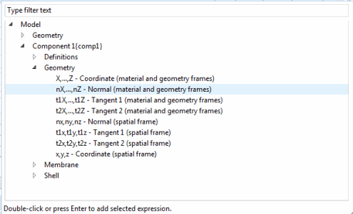
	The contact normal can be visualized by plotting <pair_tag>.n<coord_label>. For example, the variable p1.nx gives the x-component of the spatial normal used by contact pair p1. Plotting the contact normal vector can be useful to verify that contact normal for a source and destination point toward each other.

Visualizing the Orientation of Boundaries

In 2D, a boundary is represented by a line. If you follow the line from its start point to its endpoint, the positive normal points to the left. The line orientations can be visualized by selecting the checkbox in the appropriate node under .

In 3D, the rules for the orientation of a boundary are more complicated. In general, you have to visualize the normals, in order to check its orientation. This can be done in different ways:

•

For a mesh without physics, you will need to use the general result presentation tools. Follow these steps:

Run for an arbitrary study in order to create data for result presentation.

Add a under .

Add an plot to the new plot group.

In the (

) dialog, select the geometry normal.

•

When working with the Shell or Membrane interfaces, select in the settings for the interface. You will then see the physics normals plotted if you select a material model like in the Model Builder.

Contact Between Physics Interfaces

Contact can seamlessly be modeled between all applicable structural mechanics interfaces. Equations are only added by and nodes with a selection that intersects the destination boundaries of a pair. Some properties, such as contact surface offset, can, however, be added as long as either a source or a destination boundary is applicable. nodes in physics interfaces defined on boundaries, for example in the Shell interface, automatically account for the assigned thickness on both source and destination boundaries.

Source Selection Outside Physics Interfaces

In most cases, the source and destination boundaries belong to the same physics interface. However, the source side only needs to have a mesh and can optionally have one or more physics interfaces attached to it.

If the source boundary is not part of a physics interface with a or node, the contact mapping uses only the current location of the mesh, ignoring any physical properties that may exist there. In this case, the physics has no control of the contact normal used by the source boundary. Care must therefore be taken to ensure that the contact normal of the source and destination points toward each other for the contact detection to work.

There are two main scenarios where you may want to use a source selection that is not in the current physics interface:

Fixed Rigid Wall

If one side of a contact pair can be considered as rigid and fixed in space, then it is sufficient to add a meshed boundary at that location without any physics.

Moving Rigid Wall


	Since the source boundary only requires a mesh, Shell, Layered Shell, and Membrane interfaces are in fact automatically included in the contact analysis when a general contact pair is used, even though they do not support the General Contact node. However, contact is detected only with the meshed boundary and only in the direction of the contact normal.