|
|
|
|
1
|
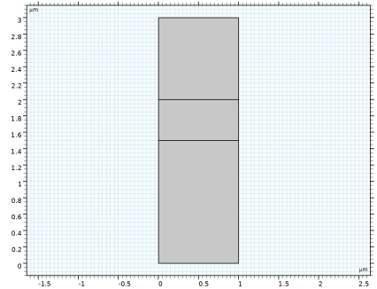
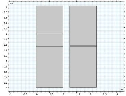
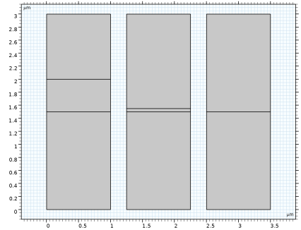
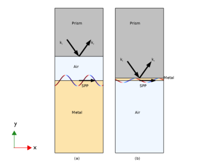
In the Model Wizard window, Use two physics interfaces to simulate the Otto and Kretschmann configurations independently, and another physics interface to calculate the angle phase matching.
|
|
2
|
click
|
|
3
|
In the Select Physics tree, select Optics > Wave Optics > Electromagnetic Waves, Frequency Domain (ewfd).
|
|
4
|
Click Add.
|
|
5
|
Click Add, to add the second physics interface.
|
|
6
|
Click Add, to add the third physics interface.
|
|
7
|
Click
|
|
8
|
In the Select Study tree, select Preset Studies for Selected Physics Interfaces > Wavelength Domain.
|
|
9
|
Click
|
|
1
|
|
2
|
|
3
|
|
1
|
|
2
|
|
1
|
|
2
|
|
3
|
|
4
|
|
5
|
Click to expand the Layers section. In the table, enter the following settings:
|
|
6
|
|
1
|
|
2
|
|
3
|
|
4
|
Locate the Layers section. In the table, enter the following settings:
|
|
5
|
Click
|
|
6
|
|
1
|
|
2
|
|
3
|
|
4
|
|
5
|
|
6
|
Locate the Layers section. In the table, enter the following settings:
|
|
7
|
Click
|
|
8
|
|
1
|
|
2
|
Go to the Add Material window.
|
|
3
|
In the tree, select Optical > Inorganic Materials > Ag - Silver > Experimental data: bulk, thick film > Ag (Silver) (Johnson and Christy 1972: n,k 0.188-1.94 um).
|
|
4
|
Right-click and choose Add to Component 1 (comp1).
|
|
5
|
|
6
|
Right-click and choose Add to Component 1 (comp1).
|
|
1
|
|
2
|
|
1
|
|
2
|
|
4
|
Locate the Material Contents section. In the table, enter the following settings:
|
|
1
|
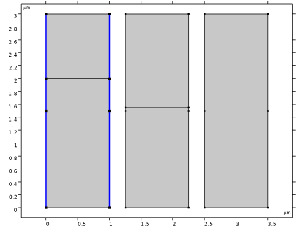
In the Model Builder window, under Component 1 (comp1) click Electromagnetic Waves, Frequency Domain (ewfd).
|
|
2
|
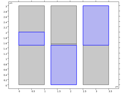
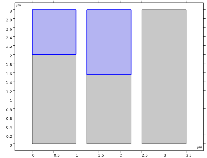
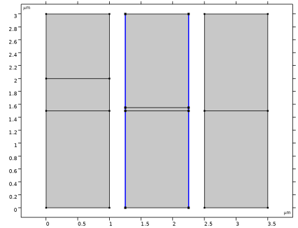
In the Settings window for Electromagnetic Waves, Frequency Domain, locate the Domain Selection section.
|
|
3
|
Click
|
|
1
|
|
3
|
|
4
|
|
5
|
|
6
|
|
7
|
|
1
|
|
2
|
|
3
|
Click
|
|
5
|
|
1
|
|
3
|
|
4
|
|
5
|
|
1
|
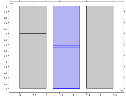
In the Model Builder window, under Component 1 (comp1) click Electromagnetic Waves, Frequency Domain 2 (ewfd2).
|
|
2
|
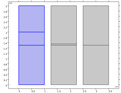
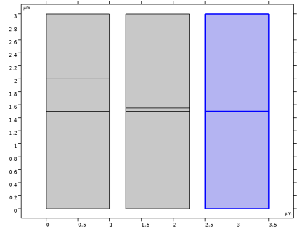
In the Settings window for Electromagnetic Waves, Frequency Domain, locate the Domain Selection section.
|
|
3
|
Click
|
|
1
|
|
3
|
|
4
|
|
5
|
|
6
|
|
7
|
|
1
|
|
2
|
|
3
|
Click
|
|
5
|
|
1
|
|
3
|
|
4
|
|
5
|
|
1
|
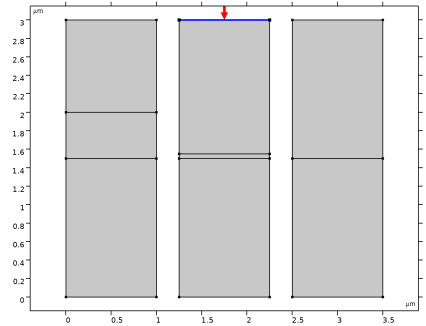
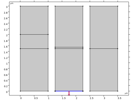
In the Model Builder window, under Component 1 (comp1) click Electromagnetic Waves, Frequency Domain 3 (ewfd3).
|
|
2
|
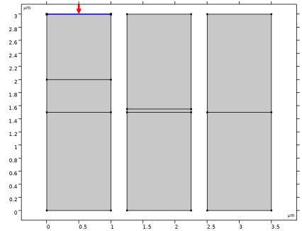
In the Settings window for Electromagnetic Waves, Frequency Domain, locate the Domain Selection section.
|
|
3
|
Click
|
|
1
|
|
3
|
|
4
|
|
1
|
|
2
|
|
3
|
Click
|
|
5
|
|
1
|
|
2
|
|
3
|
Select the Resolve wave in lossy media checkbox.
|
|
4
|
Locate the Electromagnetic Waves, Frequency Domain 2 (ewfd2) section. Select the Resolve wave in lossy media checkbox.
|
|
5
|
Locate the Electromagnetic Waves, Frequency Domain 3 (ewfd3) section. Select the Resolve wave in lossy media checkbox.
|
|
6
|
|
1
|
|
2
|
|
1
|
|
2
|
|
3
|
|
4
|
Locate the Physics and Variables Selection section. In the Solve for column of the table, under Component 1 (comp1), clear the checkboxes for Electromagnetic Waves, Frequency Domain 2 (ewfd2) and Electromagnetic Waves, Frequency Domain 3 (ewfd3). This study simulates the Otto configuration only.
|
|
5
|
|
6
|
Click
|
|
9
|
Click
|
|
10
|
|
11
|
|
12
|
|
13
|
Click Add.
|
|
14
|
|
1
|
|
2
|
Go to the Add Study window.
|
|
3
|
Find the Studies subsection. In the Select Study tree, select Preset Studies for Selected Physics Interfaces > Wavelength Domain.
|
|
4
|
Right-click and choose Add Study.
|
|
5
|
|
1
|
|
2
|
|
3
|
|
4
|
Locate the Physics and Variables Selection section. In the Solve for column of the table, under Component 1 (comp1), clear the checkboxes for Electromagnetic Waves, Frequency Domain (ewfd) and Electromagnetic Waves, Frequency Domain 3 (ewfd3).
|
|
5
|
|
6
|
Click
|
|
9
|
Click
|
|
10
|
|
11
|
|
12
|
|
13
|
Click Add.
|
|
14
|
|
1
|
|
2
|
Go to the Add Study window.
|
|
3
|
Find the Studies subsection. In the Select Study tree, select Preset Studies for Selected Physics Interfaces > Wavelength Domain.
|
|
4
|
Right-click and choose Add Study.
|
|
5
|
|
1
|
|
2
|
|
3
|
|
4
|
Locate the Physics and Variables Selection section. In the Solve for column of the table, under Component 1 (comp1), clear the checkboxes for Electromagnetic Waves, Frequency Domain (ewfd) and Electromagnetic Waves, Frequency Domain 2 (ewfd2).
|
|
1
|
|
2
|
|
3
|
|
4
|
|
5
|
Locate the Physics and Variables Selection section. In the Solve for column of the table, under Component 1 (comp1), clear the checkboxes for Electromagnetic Waves, Frequency Domain (ewfd) and Electromagnetic Waves, Frequency Domain 2 (ewfd2).
|
|
1
|
|
2
|
|
3
|
|
1
|
|
2
|
|
3
|
Click
|
|
1
|
|
2
|
|
3
|
|
1
|
|
2
|
|
3
|
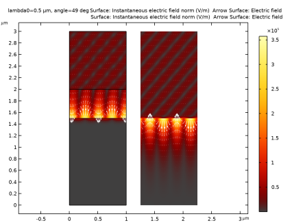
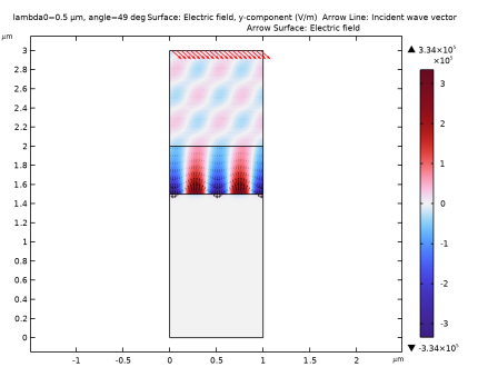
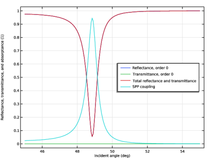
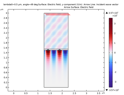
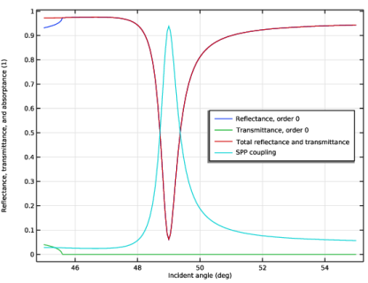
From the Parameter value (angle (deg)) list, choose 49. At this angle maximum absorption occurs, as will be shown in the next figure.
|
|
1
|
|
2
|
|
3
|
|
4
|
|
5
|
|
1
|
|
2
|
|
1
|
|
2
|
|
3
|
|
4
|
|
5
|
|
6
|
Locate the Coloring and Style section.
|
|
7
|
|
1
|
|
1
|
|
2
|
|
3
|
|
4
|
|
5
|
Locate the Arrow Positioning section. Find the X grid points subsection. In the Points text field, type 40.
|
|
6
|
|
7
|
Locate the Coloring and Style section.
|
|
8
|
|
9
|
|
10
|
|
11
|
|
1
|
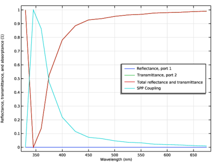
In the Model Builder window, under Results click Reflectance, Transmittance, and Absorptance (ewfd).
|
|
2
|
In the Settings window for 1D Plot Group, type Reflectance, Transmittance, and SPP Coupling, Otto (ewfd) in the Label text field.
|
|
3
|
|
1
|
In the Model Builder window, expand the Reflectance, Transmittance, and SPP Coupling, Otto (ewfd) node, then click Global 1.
|
|
2
|
|
4
|
|
1
|
|
2
|
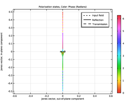
In the Settings window for 1D Plot Group, type Polarization Plot, Otto (ewfd) in the Label text field.
|
|
3
|
|
4
|
|
1
|
|
2
|
|
3
|
|
1
|
|
2
|
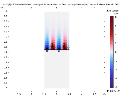
In the Settings window for 2D Plot Group, type Electric Field, Kretschmann (ewfd2) in the Label text field.
|
|
3
|
|
1
|
In the Model Builder window, expand the Electric Field, Kretschmann (ewfd2) node, then click Surface 1.
|
|
2
|
|
3
|
|
4
|
|
5
|
|
1
|
|
2
|
|
3
|
|
4
|
|
5
|
|
6
|
Locate the Coloring and Style section.
|
|
7
|
|
1
|
|
1
|
In the Model Builder window, right-click Electric Field, Kretschmann (ewfd2) and choose Arrow Surface.
|
|
2
|
|
3
|
|
4
|
|
5
|
Locate the Arrow Positioning section. Find the X grid points subsection. In the Points text field, type 40.
|
|
6
|
|
7
|
Locate the Coloring and Style section.
|
|
8
|
|
9
|
|
10
|
|
11
|
|
12
|
|
1
|
In the Model Builder window, under Results click Reflectance, Transmittance, and Absorptance (ewfd2).
|
|
2
|
In the Settings window for 1D Plot Group, type Reflectance, Transmittance, and SPP Coupling, Kretschmann (ewfd2) in the Label text field.
|
|
3
|
|
1
|
In the Model Builder window, expand the Reflectance, Transmittance, and SPP Coupling, Kretschmann (ewfd2) node, then click Global 1.
|
|
2
|
|
4
|
|
1
|
|
2
|
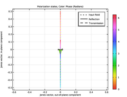
In the Settings window for 1D Plot Group, type Polarization Plot, Kretschmann (ewfd2) in the Label text field.
|
|
3
|
|
4
|
|
1
|
|
2
|
In the Settings window for 2D Plot Group, type Instantaneous Electric Field Norm in the Label text field.
|
|
3
|
|
1
|
|
2
|
|
3
|
|
4
|
|
1
|
In the Model Builder window, right-click Instantaneous Electric Field Norm and choose Arrow Surface.
|
|
2
|
|
3
|
|
4
|
|
5
|
Locate the Arrow Positioning section. Find the X grid points subsection. In the Points text field, type 30.
|
|
6
|
|
7
|
Locate the Coloring and Style section.
|
|
8
|
|
9
|
|
1
|
In the Model Builder window, under Results > Instantaneous Electric Field Norm right-click Surface 1 and choose Duplicate.
|
|
2
|
|
3
|
|
4
|
|
5
|
|
6
|
|
1
|
In the Model Builder window, under Results > Instantaneous Electric Field Norm right-click Arrow Surface 1 and choose Duplicate.
|
|
2
|
|
3
|
|
4
|
|
5
|
|
6
|
|
7
|
|
8
|
|
1
|
|
2
|
|
3
|
|
1
|
|
2
|
|
3
|
|
1
|
|
2
|
|
3
|
|
4
|
|
5
|
|
1
|
|
2
|
|
3
|
|
4
|
|
5
|
Locate the Arrow Positioning section. Find the X grid points subsection. In the Points text field, type 40.
|
|
6
|
|
7
|
Locate the Coloring and Style section.
|
|
8
|
|
9
|
|
10
|
|
1
|
In the Model Builder window, under Results click Reflectance, Transmittance, and Absorptance (ewfd3).
|
|
2
|
In the Settings window for 1D Plot Group, type Reflectance, Transmittance, and SPP Coupling (ewfd3) in the Label text field.
|
|
3
|
|
1
|
In the Model Builder window, expand the Reflectance, Transmittance, and SPP Coupling (ewfd3) node, then click Global 1.
|
|
2
|
|
4
|
|
1
|
|
2
|
|
3
|
|
4
|
|
1
|
|
2
|
|
3
|
|
4
|
|
1
|
|
2
|
|
3
|
|
1
|
|
2
|
|
3
|
|
4
|
|
5
|
Locate the Parameters section. In the table, enter the following settings:
|
|
6
|
Locate the Expressions section. In the table, enter the following settings:
|
|
7
|
|
1
|
Go to the Evaluation Group 1 window.
|
|
2
|
Click the Table Graph button in the window toolbar.
|
|
1
|
|
2
|
|
3
|
|
4
|
|
5
|
|
1
|
|
2
|
|
3
|
Locate the Plot Settings section.
|
|
4
|
|
5
|