|
|
|


|
1
|
|
2
|
In the Select Physics tree, select Optics > Wave Optics > Electromagnetic Waves, Boundary Elements (ebem).
|
|
3
|
Click Add.
|
|
4
|
Click
|
|
5
|
|
6
|
Click
|
|
1
|
|
2
|
|
1
|
|
2
|
|
3
|
In the Settings window for Variables, type Spherical Bessel Function of the First Kind in the Label text field.
|
|
4
|
Locate the Variables section. In the table, enter the following settings:
|
|
1
|
|
2
|
In the Settings window for Variables, type Spherical Bessel Function of the Second Kind in the Label text field.
|
|
3
|
Locate the Variables section. In the table, enter the following settings:
|
|
1
|
|
2
|
In the Settings window for Variables, type Spherical Hankel Function of the Second Kind in the Label text field.
|
|
3
|
Locate the Variables section. In the table, enter the following settings:
|
|
1
|
|
2
|
|
3
|
Locate the Variables section. In the table, enter the following settings:
|
|
1
|
|
2
|
|
3
|
Locate the Variables section. In the table, enter the following settings:
|
|
1
|
|
2
|
|
3
|
Locate the Variables section. In the table, enter the following settings:
|
|
1
|
|
2
|
|
3
|
|
1
|
|
2
|
|
3
|
|
4
|
|
5
|
|
6
|
Select the zx-plane: remove y<0 checkbox.
|
|
7
|
|
1
|
In the Model Builder window, under Component 1 (comp1) right-click Materials and choose Blank Material.
|
|
2
|
|
3
|
|
4
|
Locate the Material Contents section. In the table, enter the following settings:
|
|
1
|
In the Model Builder window, under Component 1 (comp1) click Electromagnetic Waves, Boundary Elements (ebem).
|
|
2
|
In the Settings window for Electromagnetic Waves, Boundary Elements, locate the Domain Selection section.
|
|
3
|
|
4
|
|
5
|
|
6
|
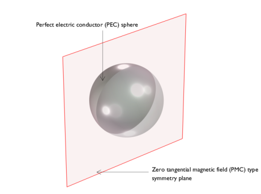
Click to expand the Symmetry section. From the Condition for the y = y0 plane list, choose Zero tangential magnetic field (PMC).
|
|
1
|
|
2
|
|
3
|
|
1
|
|
2
|
|
3
|
Click
|
|
1
|
|
2
|
|
3
|
|
4
|
|
1
|
|
2
|
|
4
|
Locate the Expressions section. In the table, enter the following settings:
|
|
5
|
Click
|
|
1
|
|
2
|
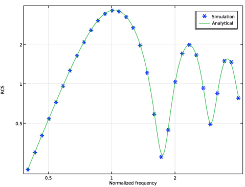
In the Settings window for 1D Plot Group, type Simulated and Analytically Calculated RCS in the Label text field.
|
|
3
|
|
4
|
|
5
|
Locate the Plot Settings section.
|
|
6
|
|
7
|
|
1
|
|
3
|
|
4
|
|
5
|
|
6
|
Click to expand the Coloring and Style section. Find the Line style subsection. From the Line list, choose None.
|
|
7
|
|
8
|
|
9
|
|
1
|
In the Model Builder window, right-click Simulated and Analytically Calculated RCS and choose Table Graph.
|
|
2
|
|
3
|
Select the Show legends checkbox.
|
|
4
|
|
6
|
|
7
|
|
8
|
|
1
|
|
2
|
|
3
|
|
4
|
|
5
|
|
6
|
|
7
|
|
8
|
|
9
|
|
10
|
|
11
|
|
1
|
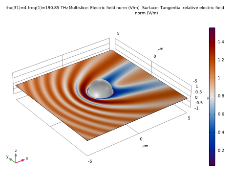
In the Model Builder window, expand the Results > Electric Field, Domains (ebem) node, then click Multislice 1.
|
|
2
|
|
3
|
|
4
|
|
5
|
|
1
|
|
2
|
|
3
|
|
4
|
|
1
|
|
2
|
|
3
|
|
4
|
|
1
|
|
2
|
|
3
|
|
1
|
|
2
|
|
3
|
|
4
|
 ,
,