|
|
|
 ,
,

|
1
|
|
2
|
In the Select Physics tree, select Optics > Wave Optics > Electromagnetic Waves, Frequency Domain (ewfd).
|
|
3
|
Click Add.
|
|
4
|
Click
|
|
5
|
|
6
|
Click
|
|
1
|
|
2
|
|
3
|
Click
|
|
4
|
Browse to the model’s Application Libraries folder and double-click the file optically_anisotropic_waveguide_parameters.txt.
|
|
1
|
|
2
|
|
3
|
|
1
|
|
2
|
|
3
|
|
4
|
|
1
|
|
2
|
|
3
|
|
4
|
|
5
|
|
6
|
Click
|
|
7
|
|
1
|
In the Model Builder window, under Component 1 (comp1) > Electromagnetic Waves, Frequency Domain (ewfd) click Wave Equation, Electric 1.
|
|
2
|
|
3
|
|
1
|
In the Model Builder window, under Component 1 (comp1) right-click Materials and choose Blank Material.
|
|
2
|
|
3
|
Locate the Material Contents section. In the table, enter the following settings:
|
|
1
|
|
2
|
|
4
|
Locate the Material Contents section. In the table, enter the following settings:
|
|
1
|
|
2
|
|
3
|
From the list, choose User-controlled mesh.
|
|
1
|
|
2
|
|
3
|
Click the Predefined button.
|
|
1
|
|
2
|
|
3
|
|
4
|
Click
|
|
1
|
|
2
|
In the Settings window for Study, type Study - Diagonal Transverse Anisotropy in the Label text field.
|
|
1
|
|
2
|
|
3
|
Click
|
|
1
|
|
2
|
|
3
|
|
4
|
|
5
|
|
6
|
Click to expand the Filtering and Sorting section. Find the Sorting subsection. Select the Mode following checkbox.
|
|
7
|
|
1
|
In the Model Builder window, expand the Results > Electric Field (ewfd) node, then click Electric Field (ewfd).
|
|
2
|
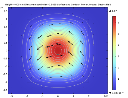
In the Settings window for 2D Plot Group, type Power and Electric Field - Diagonal Transverse Anisotropy in the Label text field.
|
|
3
|
|
1
|
|
2
|
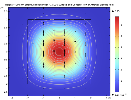
In the Settings window for Surface, click Replace Expression in the upper-right corner of the Expression section. From the menu, choose Component 1 (comp1) > Electromagnetic Waves, Frequency Domain > Energy and power > Power flow, time average - W/m² > ewfd.Poavz - Power flow, time average, z-component.
|
|
1
|
In the Model Builder window, right-click Power and Electric Field - Diagonal Transverse Anisotropy and choose Arrow Surface.
|
|
2
|
In the Settings window for Arrow Surface, click Replace Expression in the upper-right corner of the Expression section. From the menu, choose Component 1 (comp1) > Electromagnetic Waves, Frequency Domain > Electric > ewfd.Ex,ewfd.Ey - Electric field.
|
|
3
|
Locate the Arrow Positioning section. Find the X grid points subsection. In the Points text field, type 30.
|
|
4
|
|
5
|
|
1
|
|
2
|
In the Settings window for Contour, click Replace Expression in the upper-right corner of the Expression section. From the menu, choose ewfd.Poavz - Power flow, time average, z-component - W/m².
|
|
3
|
|
4
|
|
5
|
Clear the Color legend checkbox.
|
|
1
|
|
2
|
|
3
|
|
4
|
|
5
|
|
6
|
|
7
|
In the Title text area, type Height=eval(height,nm) nm Effective mode index=eval(ewfd.neff) Surface and Contour: Power Arrows: Electric field.
|
|
8
|
Clear the Parameter indicator text field.
|
|
9
|
|
10
|
|
1
|
|
2
|
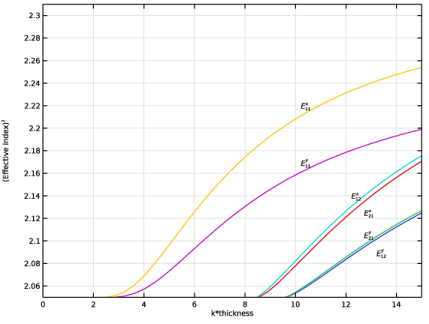
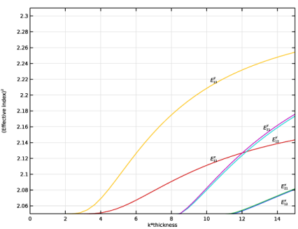
In the Settings window for 1D Plot Group, type Dispersion Curves - Diagonal Transverse Anisotropy in the Label text field.
|
|
3
|
Locate the Data section. From the Dataset list, choose Study - Diagonal Transverse Anisotropy/Parametric Solutions 1 (sol2).
|
|
4
|
|
1
|
|
2
|
|
4
|
|
5
|
|
6
|
|
7
|
|
1
|
|
2
|
|
3
|
|
4
|
|
5
|
Locate the Plot Settings section.
|
|
6
|
|
7
|
|
8
|
|
9
|
|
10
|
|
11
|
|
12
|
|
1
|
|
2
|
|
3
|
|
4
|
|
5
|
|
6
|
|
7
|
|
1
|
|
2
|
|
3
|
|
4
|
|
1
|
|
2
|
|
3
|
|
4
|
|
5
|
|
1
|
|
2
|
|
3
|
|
4
|
|
5
|
|
1
|
|
2
|
|
3
|
|
4
|
|
5
|
|
1
|
|
2
|
|
3
|
|
4
|
|
1
|
|
2
|
|
3
|
|
1
|
|
2
|
|
3
|
|
4
|
|
5
|
|
1
|
In the Model Builder window, under Component 1 (comp1) > Electromagnetic Waves, Frequency Domain (ewfd) right-click Wave Equation, Electric 1 and choose Duplicate.
|
|
2
|
In the Settings window for Wave Equation, Electric, type Wave Equation, Electric 2 - Rotated in the Label text field.
|
|
3
|
Locate the Coordinate System Selection section. From the Coordinate system list, choose Rotated System 2 (sys2).
|
|
1
|
In the Model Builder window, under Study - Diagonal Transverse Anisotropy click Step 1: Mode Analysis.
|
|
2
|
|
3
|
Select the Modify model configuration for study step checkbox.
|
|
4
|
|
5
|
In the tree, select Component 1 (comp1) > Electromagnetic Waves, Frequency Domain (ewfd) > Wave Equation, Electric 2 - Rotated.
|
|
6
|
Right-click and choose Disable.
|
|
1
|
|
2
|
Go to the Add Study window.
|
|
3
|
Find the Studies subsection. In the Select Study tree, select Preset Studies for Selected Physics Interfaces > Mode Analysis.
|
|
4
|
Click the Add Study button in the window toolbar.
|
|
1
|
|
2
|
|
3
|
|
4
|
Locate the Filtering and Sorting section. Find the Sorting subsection. Select the Mode following checkbox.
|
|
5
|
|
6
|
|
1
|
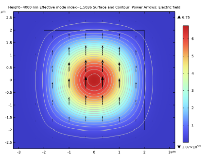
In the Settings window for 2D Plot Group, type Power and Electric Field - Off-Diagonal Longitudinal Anisotropy in the Label text field.
|
|
2
|
|
1
|
In the Model Builder window, under Results > Power and Electric Field - Diagonal Transverse Anisotropy, Ctrl-click to select Arrow Surface 1 and Contour 1.
|
|
2
|
Right-click and choose Copy.
|
|
1
|
|
2
|
|
3
|
|
4
|
|
5
|
|
6
|
|
7
|
In the Title text area, type Height=eval(height,nm) nm Effective mode index=eval(ewfd.neff) Surface and Contour: Power Arrows: Electric field.
|
|
8
|
|
1
|
In the Model Builder window, right-click Dispersion Curves - Diagonal Transverse Anisotropy and choose Duplicate.
|
|
2
|
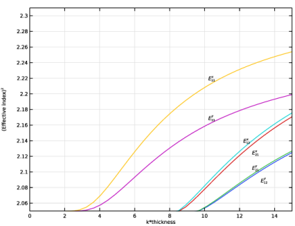
In the Settings window for 1D Plot Group, type Dispersion Curves - Off-Diagonal Longitudinal Anisotropy in the Label text field.
|
|
3
|
Locate the Data section. From the Dataset list, choose Study - Off-Diagonal Longitudinal Anisotropy/Parametric Solutions 2 (sol40).
|
|
4
|
|
1
|
In the Model Builder window, expand the Dispersion Curves - Off-Diagonal Longitudinal Anisotropy node, then click Annotation 1.
|
|
2
|
|
3
|
|
1
|
|
2
|
|
3
|
|
4
|
|
1
|
|
2
|
|
3
|
|
4
|
|
5
|
|
1
|
|
2
|
|
3
|
|
4
|
|
5
|
|
1
|
|
2
|
|
3
|
|
4
|
|
5
|
|
1
|
|
2
|
|
3
|
|
4
|
|
5
|
|
6
|