COMSOL 6.4 - Postbuckling Analysis of a Hinged Cylindrical Shell

PDF

Postbuckling Analysis of a Hinged Cylindrical Shell

Buckling is a phenomenon that can cause sudden failure of a structure.

A linear buckling analysis predicts the critical buckling load. Such an analysis, however, does not give any information about what happens at loads higher than the critical load. It also often overpredicts the load-carrying capacity of the structure. Tracing the solution after the critical load is called a postbuckling analysis.

In order to accurately determine the critical buckling load or predict the postbuckling behavior, you can use the nonlinear solver and ramp up the applied load to compute the structure deformation. The buckling load can then be based on when a certain, not acceptable, deformation is reached.

Once the critical buckling load has been reached, it can happen that the structure undergoes a sudden large deformation into a new stable configuration. This is known as a snap-through phenomenon. A snap-through process cannot be simulated using prescribed load in a standard nonlinear static solver because the problem becomes numerically singular. Physically speaking, it is a highly transient problem as the structure “jumps” from one state to another. For simple cases with a single point load, it is often possible to replace the point load with a prescribed displacement and then measure the reaction force instead.

For more general problems, the postbuckling solution must however be tracked using more sophisticated methods, as shown in this example.

Figure 1 shows the variation of load versus the displacement for such a difficult case. It illustrates the possible computational problem by using either a load control (path A) or a displacement control (path B).

Figure 1: Load versus displacement in snap-through buckling.

The shell structure in this example has a behavior similar to this.

Model Definition

The model studied here is a benchmark for a hinged cylindrical panel subjected to a point load at its center; see Ref. 1.

•

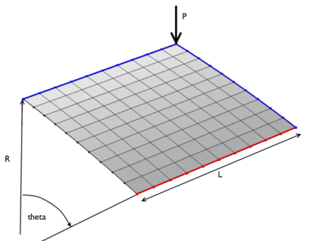
The radius of the cylinder is R = 2.54 m and all edges have a length of 2L = 0.508 m. The angular span of the panel is thus 0.2 radians. The panel thickness is th = 6.35 mm.

•

The straight edges are hinged.

•

In the study, the variation of the panel center vertical displacement with respect to the change of the applied load is of interest.

Due to the double symmetry, only one quarter of the geometry is modeled as shown in Figure 2. The blue lines show the symmetry edge conditions, while the red line shows the location of the hinged edge condition.

Figure 2: Problem description.

In general, you should be careful when using symmetry in buckling problems, because nonsymmetric solutions may exist.

In Figure 3 you can see the applied load as a function of the panel center displacement. The figure shows clearly a nonunique solution for a given applied load (between -400 N to 600 N) or a given displacement (between 14.4 mm and 17 mm).

Figure 3: Applied load versus panel center displacement.

As shown in Table 1, the results agree well with the target data from Ref. 1.

Table 1: Comparison between target and computed data.
Applied Load (N)	Displacement target (mm)	Displacement computed (mm)
155.1	1.846	1.871
574.2	11.904	12.054
485.1	15.501	15.56
24.9	17.008	17.029
-300.3	14.520	14.537
-381.3	16.961	16.769
-1.8	24.824	24.809
1469.4	33.388	33.341

Notes About the COMSOL Implementation

The main feature of this model is that a limit point instability occurs at the buckling load. Neither a load control, nor a point displacement control, would be able to track the jump between the stable solution paths (see Figure 1). To solve this type of problem you can use different approaches:

•

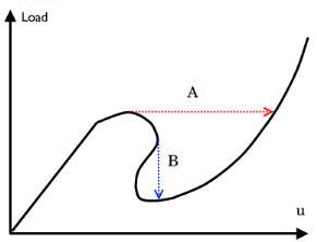
Find a proper parameter that increases monotonically. Then, use a node where the load is made a function of this monotonically increasing parameter. This is the approach used in this example. In this case, a good such parameter is the average of the displacement in the direction of the applied force. You use a nonlocal average coupling to measure the displacement and then add a global equation to compute the appropriate point load for each prescribed parameter value. There is no general way to determine which controlling parameter to use, so it is necessary to use some physical insight.

•

Use an arc length method. The Application Library example Postbuckling Analysis Using an Incremental Arc Length Method demonstrates this approach. It is useful if you cannot find a suitable monotonically increasing control parameter.

1. K.Y. Sze, X.H. Liua, and S.H. Lob, “Popular Benchmark Problems for Geometric Nonlinear Analysis of Shells,” Finite Element in Analysis and Design, vol. 40, issue 11, pp. 1551–1569, 2004.

Structural_Mechanics_Module/Verification_Examples/postbuckling_shell

Modeling Instructions

From the menu, choose .

In the window, click

.

1

In the window, click

.

2

In the tree, select > .

3

4

5

In the tree, select > .

6

Global Definitions

1

In the window, under click .

2

In the window for , locate the section.

3

In the table, enter the following settings:


Name	Expression	Value	Description
R	2540[mm]	2.54 m	Panel radius
L	254[mm]	0.254 m	Panel length
thic	6.35[mm]	0.00635 m	Panel thickness
theta	0.1[rad]	0.1 rad	Panel section angle
E0	3.103[GPa]	3.103E9 Pa	Young's modulus
nu0	0.3	0.3	Poisson's ratio
disp	0	0	Displacement parameter

Work Plane 1 (wp1)

1

In the toolbar, click

.

2

In the window for , locate the section.

3

From the list, choose .

4

Work Plane 1 (wp1) > Line Segment 1 (ls1)

1

In the toolbar, click

and choose .

2

In the window for , locate the section.

3

From the list, choose .

4

Locate the section. From the list, choose .

5

Locate the section. In the text field, type R.

6

Locate the section. In the text field, type L and to R.

7

Revolve 1 (rev1)

1

In the window, right-click and choose .

2

In the window for , locate the section.

3

Click the button.

4

In the text field, type theta.

5

Locate the section. Find the subsection. In the text field, type 1.

6

In the text field, type 0.

7

button in the toolbar.

Average 1 (aveop1)

1

In the toolbar, click

and choose .

2

In the window for , locate the section.

3

From the list, choose .

4

Select Boundary 1 only.

Integration 1 (intop1)

1

In the toolbar, click

and choose .

2

In the window for , locate the section.

3

From the list, choose .

4

Select Point 4 only.

1

In the toolbar, click

.

2

In the window for , locate the section.

3

In the table, enter the following settings:


Name	Expression	Unit
w_center	-intop1(w)	m

Thickness and Offset 1

1

In the window, under > click .

2

In the window for , locate the section.

3

In the d0 text field, type thic.

1

In the toolbar, click

and choose .

2

Select Edges 3 and 4 only.

1

In the toolbar, click

and choose .

2

Select Edge 2 only.

1

In the toolbar, click

and choose .

2

Select Point 4 only.

Apply 1/4th of the total load because of the double symmetry used in this model.

3

In the window for , locate the section.

4

Specify the FP vector as


0	x
0	y
-P/4	z

5

button in the toolbar.

6

In the dialog, in the tree, select the checkbox for the node > .

7

Global Equations 1 (ODE1)

1

In the toolbar, click

and choose .

2

In the window for , locate the section.

3

In the table, enter the following settings:


Name	f(u,ut,utt,t) (1)	Initial value (u_0) (1)	Initial value (ut_0) (1/s)	Description
P	aveop1(-w)-disp	0	0	Force at shell center

4

Locate the section. Click

.

5

In the dialog, type force in the text field.

6

In the tree, select > .

7

8

In the window for , locate the section.

9

10

In the dialog, type displacement in the text field.

11

In the tree, select > .

12

Material 1 (mat1)

1

In the window, under right-click and choose .

2

In the window for , locate the section.

3

In the table, enter the following settings:


Property	Variable	Value	Unit	Property group
Young’s modulus	E	E0	Pa	Young’s modulus and Poisson’s ratio
Poisson’s ratio	nu	nu0	1	Young’s modulus and Poisson’s ratio
Density	rho	0	kg/m³	Basic

1

In the toolbar, click

and choose .

2

Select Boundary 1 only.

1

Right-click and choose .

2

Select Edges 1 and 2 only.

3

In the window for , locate the section.

4

In the text field, type 10.

5

Postbuckling Study

1

In the window, click .

2

In the window for , type Postbuckling Study in the text field.

Step 1: Stationary

Set up an auxiliary continuation sweep for the parameter.

1

In the window, under click .

2

In the window for , click to expand the section.

3

Select the checkbox.

4

5

In the table, enter the following settings:


Parameter name	Parameter value list
disp (Displacement parameter)	range(0,2e-4,1)

6

Locate the section. Select the checkbox.

Sometimes it is not straightforward to guess the maximum value of the parameter used. You can then instead set a stop condition for the parametric solver based on something that is known.

Solution 1 (sol1)

1

In the toolbar, click

.

2

In the window, expand the node.

3

In the window, expand the > > > node.

4

Right-click > > > > and choose .

5

In the window for , locate the section.

6

7

In the table, enter the following settings:


Stop expression	Stop if	Active	Description
comp1.w_center>0.035	True (>=1)	√	Stop expression 1

Specify that the solution is to be stored just before the stop condition is reached.

8

Locate the section. From the list, choose .

9

Clear the checkbox.

10

In the window, under > > click .

11

In the window for , click to expand the section.

12

Clear the checkbox.

13

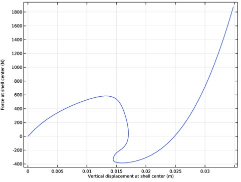
Evaluation Group: Force vs. Displacement

1

In the toolbar, click

.

2

In the window for , type Evaluation Group: Force vs. Displacement in the text field.

Point Evaluation 1

1

Right-click and choose .

2

Select Point 4 only.

3

In the window for , locate the section.

4

In the table, enter the following settings:


Expression	Unit	Description
w_center	m	Vertical displacement at shell center
P	N	Force at shell center

Evaluation Group: Force vs. Displacement

1

In the window, click .

2

In the window for , click to expand the section.

3

From the list, choose .

4

In the toolbar, click

.

Force vs. Displacement

1

In the toolbar, click

.

2

In the window for , type Force vs. Displacement in the text field.

3

Locate the section.

4

Select the checkbox. In the associated text field, type Vertical displacement at shell center (m).

5

Select the checkbox. In the associated text field, type Force at shell center (N).

1

Right-click and choose .

2

In the window for , locate the section.

3

From the list, choose .

Force vs. Displacement

1

In the window, click .

2

In the toolbar, click

.