PDF

Bracket — Eigenfrequency Analysis
Introduction
In this example, you learn how to perform an eigenfrequency analysis for an unloaded structure as well as for a prestressed structure.
When the structure is subjected to a constant external load, the stiffness generated by the stress may affect the natural frequencies of the structure. Tensile stresses tend to increase the natural frequencies, while compressive stresses tend to decrease them.
It is recommended you review the Introduction to the Structural Mechanics Module, which includes background information and discusses the bracket_basic.mph model relevant to this example.
In the Structural Mechanics Modeling chapter of the Structural Mechanics Module User’s Guide: Eigenfrequency Analysis.
Model Definition
This tutorial is an extension of the example described in the section “The Fundamentals: A Static Linear Analysis” in the Introduction to the Structural Mechanics Module.
The geometry is shown in Figure 1.
Figure 1: Geometry of the bracket.
In the first case, the natural frequencies of the unloaded bracket are studied, while in the second case it is considered how the natural frequencies are affected by a static external load. The static load is applied to the pin holes, and the left arm is under a pure compressive load while the right arm is under a pure tensile load.
Results and Discussion
Figure 2 and Figure 3 show the first six eigenmodes for the unloaded and the prestressed case, respectively. The difference in the two first mode shapes between the two load cases is significant. For the unloaded structure, there is a full symmetry, leading to the two closely spaced first eigenfrequencies. With prestress, the first eigenmodes for the two arms become distinct. The problem is no longer symmetric, since one arm is loaded in tension and the other one in compression.
The two first mode shapes consist of bending in the x direction in the bracket arms. For the unloaded case the corresponding eigenfrequencies are expected to be approximately equal because of the symmetry. For the prestressed case, there will be a difference because of stress stiffening (right arm) and stress softening (left arm).
Figure 2: Six first eigenmode shapes for the unloaded case.
Figure 3: Six first eigenmode shapes for the prestressed case.
When comparing eigenmodes, it should be noted that the modes may be computed with reversed signs. This can even happen when the same study is run twice. Note also that the magnitude of an eigenmode does not have any physical significance; that is why the default mode shape plots do not have a color legend.
In Figure 4, the stress state from the static preload is shown.
Figure 4: Equivalent stress from the preload. Note the nonlinear color scale.
In Figure 5 below, the frequency shifts in the two first eigenmodes are clearly visible.
Figure 5: The six first eigenfrequencies for the unloaded case (stars) and the prestressed case (circles).
For the unloaded case, the two first eigenfrequencies are approximately 114 Hz. They correspond to the bending mode in the x direction for the two bracket arms. For the prestressed load case, the eigenfrequencies for the bending modes are 105 Hz for the left arm and 128 Hz for the right arm. Such a frequency shift is expected since a tensile load causes stress stiffening, while a compressive load causes stress softening. The other eigenmodes are not significantly affected by the prestress.
Notes About the COMSOL Implementation
For a structural mechanics physics interface in COMSOL Multiphysics, there are two predefined study types available for eigenfrequency analysis: Eigenfrequency and Eigenfrequency, Prestressed.
The plain eigenfrequency analysis computes the natural frequencies of the unloaded structure. The contribution of any traction boundary condition is disregarded and prescribed displacement constraints are considered as having the value zero.
In the prestressed eigenfrequency analysis, a stationary analysis is first performed to take into account the different loads and nonzero displacement constraints. The resulting stress is then automatically taken into account in the stiffness used in the eigenfrequency calculation.
As a default, the Include geometric nonlinearity checkbox is selected in the Stationary study step used for computing the prestress solution. In many cases, you can choose to clear that checkbox. In this example, that would change the natural frequencies only by about 1%.
If there are no other nonlinearities in the model, you can shorten the analysis time by using an assumption about geometrical linearity, since no iterations are then needed in the first study step.
Application Library path: Structural_Mechanics_Module/Tutorials/bracket_eigenfrequency
Modeling Instructions
Application Libraries
1
From the File menu, choose Application Libraries.
2
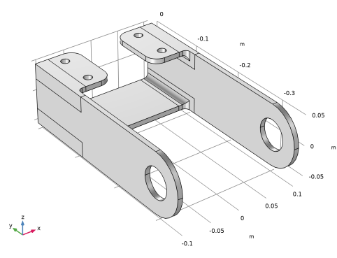
In the Application Libraries window, select Structural Mechanics Module > Tutorials > bracket_basic in the tree.
3
Add Study
1
In the Home toolbar, click  Add Study to open the Add Study window.
2
Go to the Add Study window.
3
Find the Studies subsection. In the Select Study tree, select General Studies > Eigenfrequency.
4
Click the Add Study button in the window toolbar.
5
In the Home toolbar, click  Add Study to close the Add Study window.
Study 1
Step 1: Eigenfrequency
In the Eigenfrequency study node you have the possibility to select the number of eigenfrequencies to compute, and the frequency around which you would like to search for these frequencies. By default, the eigenvalue solver finds the six lowest frequencies.
1
In the Settings window for Eigenfrequency, locate the Study Settings section.
2
Select the Desired number of eigenfrequencies checkbox. In the associated text field, type 10.
3
In the Study toolbar, click  Compute.
Results
Mode Shapes, Original
You can access the different eigenfrequency solutions in the 3D Plot Group Settings.
Note that the displacement values are normalized and have no physical significance. The normalization method can be changed in the Eigenvalue Solver node, located under the Solver Configuration node.
Modify the plot so that the first six eigenmodes are plotted side by side.
1
In the Settings window for 3D Plot Group, type Mode Shapes, Original in the Label text field.
2
Click to expand the Title section. From the Title type list, choose None.
3
Click to expand the Plot Array section. From the Array type list, choose Square.
4
In the Relative row padding text field, type 0.4.
5
In the Relative column padding text field, type 0.4.
6
Click the  Show Grid button in the Graphics toolbar.
Surface 1
1
In the Model Builder window, expand the Mode Shapes, Original node, then click Surface 1.
2
In the Settings window for Surface, click to expand the Plot Array section.
Solution Array 1
1
Right-click Surface 1 and choose Solution Array.
2
Click the  Zoom Extents button in the Graphics toolbar.
3
In the Settings window for Solution Array, locate the Plot Array section.
4
From the Array shape list, choose Square.
5
Locate the Data section. From the Eigenfrequency selection list, choose Manual.
6
In the Eigenfrequency indices (1-10) text field, type range(1,1,6).
7
In the Mode Shapes, Original toolbar, click  Plot.
Annotation 1
1
In the Model Builder window, right-click Mode Shapes, Original and choose Annotation.
2
In the Settings window for Annotation, locate the Annotation section.
3
From the Geometry level list, choose Global.
4
In the Text text field, type eval(freq) Hz.
5
Locate the Position section. In the X text field, type -0.05.
6
In the Y text field, type -0.3.
7
Locate the Coloring and Style section. Clear the Show point checkbox.
8
Click to expand the Plot Array section. Select the Manual indexing checkbox.
9
Click to expand the Advanced section. In the Precision text field, type 4.
10
In the Mode Shapes, Original toolbar, click  Plot.
Solution Array 1
In the Model Builder window, under Results > Mode Shapes, Original > Surface 1 right-click Solution Array 1 and choose Copy.
Solution Array 1
1
In the Model Builder window, right-click Annotation 1 and choose Paste Solution Array.
2
In the Mode Shapes, Original toolbar, click  Plot.
Global Evaluation 1
1
In the Results toolbar, click  Global Evaluation.
2
In the Settings window for Global Evaluation, locate the Expressions section.
3
4
Click  Evaluate.
Global Definitions
Parameters 1
1
In the Model Builder window, under Global Definitions click Parameters 1.
2
In the Settings window for Parameters, locate the Parameters section.
3
Definitions
Change reference orientation of the cylindrical system so that the loads are pointing inward and outward.
Cylindrical System 2 (sys2)
1
In the Model Builder window, expand the Component 1 (comp1) > Definitions node, then click Cylindrical System 2 (sys2).
2
In the Settings window for Cylindrical System, locate the Settings section.
3
Find the Direction of axis ϕ=0 subsection. In the table, enter the following settings:
Solid Mechanics (solid)
Boundary Load 1
1
In the Physics toolbar, click  Boundaries and choose Boundary Load.
Apply a boundary load to the bracket holes. Since the entire circumference of each hole is selected, the expression for the pressure must be truncated so that it acts only on the intended 180 degrees
2
In the Settings window for Boundary Load, locate the Boundary Selection section.
3
From the Selection list, choose Pin Holes.
4
Locate the Coordinate System Selection section. From the Coordinate system list, choose Boundary System 1 (sys1).
5
Locate the Force section. Specify the fA vector as
Add Study
1
In the Home toolbar, click  Add Study to open the Add Study window.
2
Go to the Add Study window.
The prestressed eigenfrequency analysis is available as a predefined study.
3
Find the Studies subsection. In the Select Study tree, select Preset Studies for Selected Physics Interfaces > Eigenfrequency, Prestressed.
4
Click the Add Study button in the window toolbar.
5
In the Home toolbar, click  Add Study to close the Add Study window.
Note that the newly generated study combines one stationary analysis and one eigenfrequency analysis.
Study 2
Step 2: Eigenfrequency
1
In the Settings window for Eigenfrequency, locate the Study Settings section.
2
Select the Desired number of eigenfrequencies checkbox. In the associated text field, type 10.
3
In the Search for eigenfrequencies around shift text field, type 100.
4
In the Model Builder window, click Study 2.
5
In the Settings window for Study, locate the Study Settings section.
6
Clear the Generate default plots checkbox.
7
In the Study toolbar, click  Compute.
Results
Mode Shapes, Prestressed
1
In the Model Builder window, right-click Mode Shapes, Original and choose Duplicate.
2
In the Model Builder window, click Mode Shapes, Original 1.
3
In the Settings window for 3D Plot Group, type Mode Shapes, Prestressed in the Label text field.
4
Locate the Data section. From the Dataset list, choose Study 2/Solution 2 (sol2).
5
In the Mode Shapes, Prestressed toolbar, click  Plot.
In the settings for the second plot group you can see the list of the new eigenfrequencies. You can also add them to the previous table for easy comparison with the corresponding values without preload.
Global Evaluation 1
1
In the Model Builder window, under Results > Derived Values click Global Evaluation 1.
2
In the Settings window for Global Evaluation, locate the Data section.
3
From the Dataset list, choose Study 2/Solution 2 (sol2).
4
Locate the Expressions section. In the table, enter the following settings:
5
Click  Evaluate.
Add a plot with stress and loads for the prestressed state.
Result Templates
1
In the Results toolbar, click  Result Templates to open the Result Templates window.
2
Go to the Result Templates window.
3
In the tree, select Study 2/Solution Store 1 (sol3) > Solid Mechanics > Stress (solid) and Study 2/Solution Store 1 (sol3) > Solid Mechanics > Applied Loads (solid) > Boundary Loads (solid).
4
Click the Add Result Template button in the window toolbar.
5
In the Results toolbar, click  Result Templates to close the Result Templates window.
Results
Boundary Loads (solid)
Click the  Zoom Extents button in the Graphics toolbar.
Boundary Load 1
1
In the Model Builder window, expand the Boundary Loads (solid) node.
2
Right-click Boundary Load 1 and choose Copy.
Boundary Load 1
1
In the Model Builder window, right-click Stress (solid) and choose Paste Arrow Surface.
2
In the Settings window for Arrow Surface, click to expand the Inherit Style section.
3
From the Plot list, choose Volume 1.
4
Clear the Color checkbox.
5
Clear the Color and data range checkbox.
6
Locate the Coloring and Style section. From the Arrow base list, choose Head.
Color Expression
1
In the Model Builder window, expand the Boundary Load 1 node, then click Color Expression.
2
In the Settings window for Color Expression, locate the Coloring and Style section.
3
Clear the Color legend checkbox.
Boundary Loads (solid)
In the Model Builder window, under Results right-click Boundary Loads (solid) and choose Delete.
Volume 1
1
In the Model Builder window, under Results > Stress (solid) click Volume 1.
2
In the Settings window for Volume, locate the Coloring and Style section.
3
From the Color table transformation list, choose Nonlinear.
4
Set the Color calibration parameter value to -1.4.
Stress From Static Load
1
In the Model Builder window, under Results click Stress (solid).
2
In the Settings window for 3D Plot Group, type Stress From Static Load in the Label text field.
3
Click the  Zoom Extents button in the Graphics toolbar.
4
In the Stress From Static Load toolbar, click  Plot.
Eigenfrequency Comparison
1
In the Results toolbar, click  1D Plot Group.
2
In the Settings window for 1D Plot Group, type Eigenfrequency Comparison in the Label text field.
3
Locate the Plot Settings section.
4
Select the y-axis label checkbox. In the associated text field, type Frequency [Hz].
5
Locate the Grid section. Select the Manual spacing checkbox.
6
Locate the Legend section. From the Position list, choose Upper left.
Table Graph 1
1
Right-click Eigenfrequency Comparison and choose Table Graph.
2
In the Settings window for Table Graph, locate the Data section.
3
From the x-axis data list, choose Row index.
4
From the Plot columns list, choose Manual.
5
In the Columns list, choose Frequency (Hz) and Frequency, Prestress (Hz).
6
Click to expand the Legends section. Select the Show legends checkbox.
7
Locate the Coloring and Style section. Find the Line style subsection. From the Line list, choose None.
8
Find the Line markers subsection. From the Marker list, choose Cycle.
9
In the Eigenfrequency Comparison toolbar, click  Plot.
10
Click the  y-Axis Log Scale button in the Graphics toolbar.