COMSOL 6.4 - Critical Speed of a Dual Rotor System

Dual shaft systems with intershaft bearings are becoming a standard configuration for gas turbine engines, where high power output is required. These systems consist of two coaxial rotors (shafts) running at different speeds, and interlinked through a multispool bearing. In this example, an eigenfrequency analysis is performed for such a dual rotor system to determine critical speeds. Cross-exciting vibrations through the multispool bearing couple the dynamic behavior of the two rotors.

Model Definition

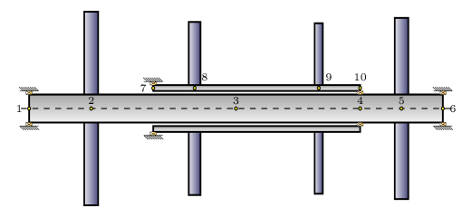
The model consists of two coaxial rotors connected through an intershaft bearing. The solid inner rotor is supported by bearings at both ends, at stations 1 and 6. The left end of the hollow outer rotor (station 7) is supported by a bearing. At the right end of the outer rotor (station 10), a multispool bearing provides mutual support between the inner and outer rotors. The rotor configuration is shown in Figure 1.

Figure 1: Rotor configuration.

Two disks are mounted on the inner rotor at stations 2 and 5. Two additional disks are mounted on the outer rotor at stations 8 and 9. Table 1 lists the positions of the stations with station 1 as reference.

Table 1: Positions of the Stations.
Station	Position	Station	Position
1	0 cm	6	50.8 cm
2	7.62 cm	7	15.24 cm
3	25.4 cm	8	20.32 cm
4	40.64 cm	9	35.56 cm
5	45.72 cm	10	40.64 cm

Table 2 lists the properties for the rotors.

Table 2: properties of the rotors.
Property	Value
Density ρ	8304 kg/m3
Young’s modulus E	206.9 GPa
Poisson’s ratio ν	0.3
Inner rotor radius r1	1.52 cm
Outer rotor inner radius r2i	1.905 cm
Outer rotor outer radius r2o	2.54 cm

Table 3 lists the properties of the mounted disks.

Table 3: Properties of the Disks.
Station	Mass	Polar moment of inertia	Diametral moment of inertia
2	4.904 kg	0.02712 kg/m2	0.01356 kg/m2
5	4.203 kg	0.02034 kg/m2	0.01017 kg/m2
8	3.327 kg	0.01469 kg/m2	0.007345 kg/m2
9	2.227 kg	0.00972 kg/m2	0.00486 kg/m2

All the bearings are isotropic. Table 4 lists their stiffnesses at different stations.

Table 4: Bearing Stiffness.
Station	Stiffness
1	27.95 MN/m
4/10	8.7598 MN/m
6	17.519 MN/m
7	17.519 MN/m

Results and Discussion

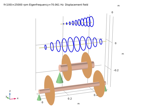
Figure 2 shows the whirl plot for the first mode (backward whirl, f = 70.1 Hz) at 25,000 rpm. To relate this plot to the rotor system, the rotors, bearings, and disks are shown beneath it.

Figure 2: Whirl plot for the first mode.

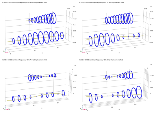
Whirl plots for other modes are shown in Figure 3. The figure shows that the inner rotor exhibits bending modes, while the outer rotor exhibits rigid body modes.

Figure 3: Mode shapes for different frequencies.

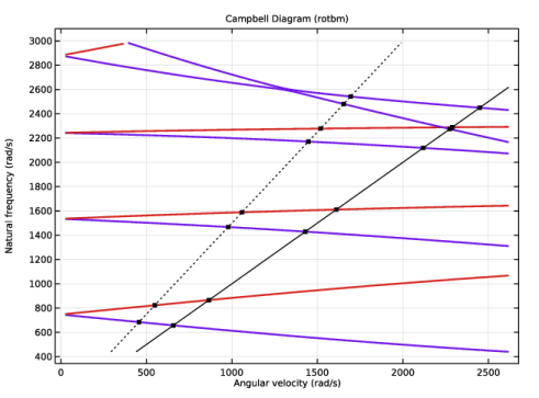
A Campbell diagram for the dual rotor system is shown in Figure 4. The two lines represent the rotational speeds of two rotors (inner and outer rotors), while the remaining lines corresponds to the eigenfrequencies of the combined rotor system. The critical speeds of the inner rotor are compared in Table 5 to the critical speeds of Ref. 1.

Table 5: Comparison of Critical Speeds for the Inner Rotor.
Mode	COMSOL (rad/s)	Ref. 1 (rad/s)
First (backward)	658	660
First (forward)	866	863
Second (backward)	1430	1423
Second (forward)	1612	1606
Third (backward)	2118	2125
Third (forward)	2270	2283

Figure 4: Campbell diagram for the rotor system.

The critical speeds of the outer rotor are compared in Table 6 to the critical speeds of Ref. 1.

Table 6: Comparison of Critical Speeds for the Outer Rotor.
Mode	COMSOL (rad/s)	Ref. 1 (rad/s)
First (backward)	685	687
First (forward)	823	822
Second (backward)	1467	1462
Second (forward)	1589	1584
Third (backward)	2171	2175
Third (forward)	2278	2274

Reference

1. J.S. Rao., Rotor Dynamics, example 8.11, pp. 266–269, New Age International (P) Limited, 2014.

Rotordynamics_Module/Verification_Examples/dual_rotors

Modeling Instructions

From the menu, choose .

New

In the window, click

Model Wizard

In the window, click

In the tree, select > > .

Click .

Click

In the tree, select > .

Click

Create a list of parameters for the geometry of the rotors.

Global Definitions

Parameters: Geometry

In the window, under click .

In the window for , type Parameters: Geometry in the text field.

Locate the section. In the table, enter the following settings:


Name	Expression	Value	Description
x1	0[cm]	0 m	Position of station 1
x2	7.62[cm]	0.0762 m	Position of station 2
x3	25.4[cm]	0.254 m	Position of station 3
x4	40.64[cm]	0.4064 m	Position of station 4
x5	45.72[cm]	0.4572 m	Position of station 5
x6	50.8[cm]	0.508 m	Position of station 6
x7	15.24[cm]	0.1524 m	Position of station 7
x8	20.32[cm]	0.2032 m	Position of station 8
x9	35.56[cm]	0.3556 m	Position of station 9
x10	40.64[cm]	0.4064 m	Position of station 10
r1	1.52[cm]	0.0152 m	Radius of the inner rotor
r2i	1.905[cm]	0.01905 m	Inner radius of the outer rotor
r2o	2.54[cm]	0.0254 m	Outer radius of the outer rotor

Create a list of parameters for the bearing properties.

Parameters: Bearing

In the toolbar, click

and choose > .

In the window for , type Parameters: Bearing in the text field.

Locate the section. In the table, enter the following settings:


Name	Expression	Value	Description
k1	27.95e6[N/m]	2.795E7 N/m	Stiffness, bearing at station 1
k4	8.7598e6[N/m]	8.7598E6 N/m	Stiffness, bearing between stations 4 and 10
k6	17.519e6[N/m]	1.7519E7 N/m	Stiffness, bearing at station 6
k7	17.519e6[N/m]	1.7519E7 N/m	Stiffness, bearing at station 7

Create a list of parameters for the material properties.

Parameters: Material

In the toolbar, click

and choose > .

In the window for , type Parameters: Material in the text field.

Locate the section. In the table, enter the following settings:


Name	Expression	Value	Description
Es	206.9[GPa]	2.069E11 Pa	Young's modulus of the rotors
rhos	8304[kg/m^3]	8304 kg/m³	Density of the rotors
nus	0.3	0.3	Poisson's ratio of the rotors
m2	4.904[kg]	4.904 kg	Mass at station 2
m5	4.203[kg]	4.203 kg	Mass at station 5
m8	3.327[kg]	3.327 kg	Mass at station 8
m9	2.227[kg]	2.227 kg	Mass at station 9
Ip2	0.02712[kg*m^2]	0.02712 kg·m²	Polar moment of inertia at station 2
Ip5	0.02034[kg*m^2]	0.02034 kg·m²	Polar moment of inertia at station 5
Ip8	0.01469[kg*m^2]	0.01469 kg·m²	Polar moment of inertia at station 8
Ip9	0.00972[kg*m^2]	0.00972 kg·m²	Polar moment of inertia at station 9
Id2	Ip2/2	0.01356 kg·m²	Diametral moment of inertia at station 2
Id5	Ip5/2	0.01017 kg·m²	Diametral moment of inertia at station 5
Id8	Ip8/2	0.007345 kg·m²	Diametral moment of inertia at station 8
Id9	Ip9/2	0.00486 kg·m²	Diametral moment of inertia at station 9

Finally, create a list of parameters for the angular speeds of the rotors.

Parameters: Angular speed

In the toolbar, click

and choose > .

In the window for , type Parameters: Angular speed in the text field.

Locate the section. In the table, enter the following settings:


Name	Expression	Value	Description
fr	1000[rpm]	16.667 1/s	Angular speed of the inner rotor
fr2	1.5*fr	25 1/s	Angular speed of the outer rotor

Now, create the lines (polygons) representing the axles of the rotors. For coaxial rotors, these lines would overlap. Here, create the lines with an offset for clarity and to facilitate making selections for various features in the instructions that follow.

Geometry 1

Polygon 1 (pol1)

In the toolbar, click

and choose .

In the window for , locate the section.

In the table, enter the following settings:


x (m)	y (m)	z (m)
x1	0	0
x2	0	0
x3	0	0
x4	0	0
x5	0	0
x6	0	0

Add the selection as for later use.

Locate the section. Find the subsection. Click .

In the dialog, type Inner Rotor in the text field.

Click .

Polygon 2 (pol2)

In the toolbar, click

and choose .

In the window for , locate the section.

In the table, enter the following settings:


x (m)	y (m)	z (m)
x7	0	6*r2o
x8	0	6*r2o
x9	0	6*r2o
x10	0	6*r2o

Add the selection as for later use.

Locate the section. Find the subsection. Click .

In the dialog, type Outer Rotor in the text field.

Click .

In the window for , click

Materials

Material 1 (mat1)

In the window, under right-click and choose .

In the window for , locate the section.

In the table, enter the following settings:


Property	Variable	Value	Unit	Property group
Young’s modulus	E	Es	Pa	Young’s modulus and Poisson’s ratio
Poisson’s ratio	nu	nus	1	Young’s modulus and Poisson’s ratio
Density	rho	rhos	kg/m³	Basic

Beam Rotor (rotbm)

In the window, under click .

In the window for , locate the section.

In the text field, type fr.

Rotor Cross Section 1

In the window, under > click .

In the window for , locate the section.

In the do text field, type 2*r1.

Rotor Cross Section 2

In the toolbar, click

and choose .

In the window for , locate the section.

From the list, choose .

Locate the section. From the list, choose .

In the do text field, type 2*r2o.

In the di text field, type 2*r2i.

Change Rotor Speed 1

In the toolbar, click

and choose .

In the window for , locate the section.

From the list, choose .

Locate the section. In the text field, type fr2.

Disk 1

In the toolbar, click

and choose .

Select Point 2 only.

In the window for , locate the section.

In the m text field, type m2.

In the Ip text field, type Ip2.

In the Id text field, type Id2.

Disk 2

In the toolbar, click

and choose .

Select Point 9 only.

In the window for , locate the section.

In the m text field, type m5.

In the Ip text field, type Ip5.

In the Id text field, type Id5.

Disk 3

In the toolbar, click

and choose .

Select Point 4 only.

In the window for , locate the section.

In the m text field, type m8.

In the Ip text field, type Ip8.

In the Id text field, type Id8.

Disk 4

In the toolbar, click

and choose .

Select Point 6 only.

In the window for , locate the section.

In the m text field, type m9.

In the Ip text field, type Ip9.

In the Id text field, type Id9.

Journal Bearing 1

In the toolbar, click

and choose .

Select Point 1 only.

In the window for , locate the section.

From the list, choose .

Specify the ku matrix as


k1	0
0	k1

Multi-Spool Bearing 1

In the toolbar, click

and choose .

Select Point 7 only.

In the window for , locate the section.

Click to select the

toggle button.

Select Point 8 only.

Locate the section. From the list, choose .

Specify the ku matrix as


k4	0
0	k4

Journal Bearing 2

In the toolbar, click

and choose .

Select Point 10 only.

In the window for , locate the section.

From the list, choose .

Specify the ku matrix as


k6	0
0	k6

Journal Bearing 3

In the toolbar, click

and choose .

Select Point 3 only.

In the window for , locate the section.

From the list, choose .

Specify the ku matrix as


k7	0
0	k7

Study 1

Now, setup a parametric sweep with the rotational speed as the swept parameter. We will also make use of the mode following functionality. To make it easier to track the different modes, it can sometimes be better to initiate the sweep with a nonzero rotational speed.

Parametric Sweep

In the toolbar, click

In the window for , locate the section.

Click

In the table, enter the following settings:


Parameter name	Parameter value list	Parameter unit
fr (Angular speed of the inner rotor)	range(250,250,25000)	rpm

Next, increase the number of desired eigenfrequencies to eight, and activate mode following for continuous tracking of the eigenfrequencies over the swept interval.

Step 1: Eigenfrequency

In the window, click .

In the window for , locate the section.

Select the checkbox. In the associated text field, type 8.

Click to expand the section. Find the subsection. Select the checkbox.

Next, increase the storage of extra eigenmodes.

Solution 1 (sol1)

In the toolbar, click

In the window, expand the node.

In the window, expand the > > > node, then click .

In the window for , locate the section.

Select the checkbox.

From the list, choose .

In the text field, type 1.

In the text field, type 1e-6.

In the toolbar, click

Follow the instructions below to create a whirl plot similar to Figure 2.

Results

Whirl (rotbm)

In the window for , locate the section.

From the list, choose .

In the window, expand the node.

Deformation

In the window, expand the > > node, then click .

In the window for , locate the section.

In the text field, type 1.5.

Disk 1

In the window, under > click .

In the window for , click to expand the section.

From the list, choose .

Disk 2

In the window, click .

In the window for , locate the section.

From the list, choose .

Disk 3

In the window, click .

In the window for , locate the section.

From the list, choose .

Disk 4

In the window, click .

In the window for , locate the section.

From the list, choose .

Journal Bearing 1

In the window, click .

In the window for , locate the section.

From the list, choose .

Journal Bearing 2

In the window, click .

In the window for , locate the section.

From the list, choose .

Journal Bearing 3

In the window, click .

In the window for , locate the section.

From the list, choose .

In the toolbar, click

Now, disable the nodes corresponding to the geometry in the group to plot only the mode shapes. These plots are shown in Figure 3.

Whirl (rotbm)

In the window, expand the > node.

Disk 1, Disk 2, Disk 3, Disk 4, Journal Bearing 1, Journal Bearing 2, Journal Bearing 3, Rotor

In the window, under > , Ctrl-click to select , , , , , , , and .

Right-click and choose .

Whirl (rotbm)

In the window, click .

In the window for , locate the section.

From the list, choose .

Click the

button in the toolbar.

In the toolbar, click

From the list, choose .

In the toolbar, click

From the list, choose .

In the toolbar, click

From the list, choose .

In the toolbar, click

You can now enable the nodes corresponding to the geometry to revert the plot to the default state.

Disk 1, Disk 2, Disk 3, Disk 4, Journal Bearing 1, Journal Bearing 2, Journal Bearing 3, Rotor

In the window, under > , Ctrl-click to select , , , , , , , and .

Right-click and choose .

Whirl (rotbm)

Click the

button in the toolbar.

The predefined Campbell diagram only shows the ω=Ω curve for the primary rotor (inner rotor). Modify the settings to add a similar curve for the outer rotor. The Campbell diagram is shown in Figure 4.

Result Templates

In the toolbar, click