


PDF

Beads-on-String Structure of Viscoelastic Filaments
Introduction
In this example, the thinning of a viscoelastic filament under the action of surface tension is studied. The evolution of the filament radius depends on the relative magnitude of capillary, viscous, and elastic stresses. The interplay of capillary and elastic stresses leads to the formation of very thin and stable filaments between drops, a so-called beads-on-a-string structure. The transformation of the filament shape can be divided into two regimes with distinct time scales. First, for times smaller than the polymer relaxation time, the beads-on-string structure develops. This is followed by exponential thinning of the threads. The fluid is expelled from the threads to the connected beads leading to almost spherical drops. The numerical results show that both transient regimes compare well with experimental measurements.
Model Definition
This example studies the evolution of a long, initially unstretched filament of Oldroyd-B fluid. The flow is considered as axisymmetric. The fluid filament is modeled as a liquid cylinder with a small perturbation of the initial radius of the cylinder, R0 (Figure 1, t = 0). The radius of the column is given by
where z is the z-coordinate and ε is the perturbation magnitude.
The fluid is a dilute solution of polymer in a Newtonian liquid with solvent of viscosity μs. The polymer is characterized by two physical parameters: the viscosity μp and the relaxation time λ.
Nondimensional Formulation
The problem is made dimensionless by using an initial radius of the cylinder, R0, surface tension coefficient σ, and fluid density ρ. The corresponding inertial-capillary time scale is
Dynamics of the filament thinning is governed by two dimensionless parameters: Deborah number and Ohnesorge number. The nondimensional polymer solution relaxation time is called the Deborah number:
The Ohnesorge number is the ratio between the inertia-capillary and viscous-capillary time scales:
where μ0 = μs + μp is the total viscosity of the polymer.
The relative importance of viscous stresses from the solvent can be characterized by the solvent viscosity ratio β = μs/μ0. The dimensionless viscosities of the solvent and the polymer contribution are ηs = β Oh and ηp = (1 − β) Oh, respectively.
Results and Discussion
Figure 1 shows the evolution of the filament at the different time steps. The results are in good agreement with the experimental and simulation results presented in Ref. 1 for the following set of the dimensionless parameters: β = 0.25, Oh = 3.16, and De = 94.9.
Figure 1: Filament profiles at 5 different dimensionless times: 0, 20, 30, 100, and 300.
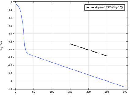
The minimum filament radius as a function of time is plotted in Figure 2. After a rapid formation of the beads-on-string structure, the figure shows the slow thinning of the thread.
Figure 2: The minimum radius of the filament as a function of time.
The rate of thinning is determined by the balance of surface tension and the elastic forces. Under the assumption of a spatially constant and slender profile, the asymptotic solution of the problem can be derived as
(1)
where r0 is an integration constant that depends on initial conditions. Figure 2 shows that minimum radius evolution curve follows the asymptotic prediction well for large times (t/τ > 40).
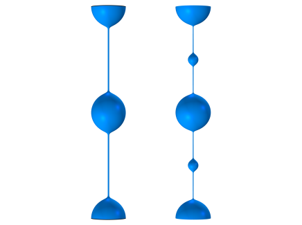
For low viscosities or high surface tensions, the formation of the satellite drops can be observed (Ref. 2). To compute the right plot in Figure 3, the finer mesh should be used.
Figure 3: Filament shapes for β = 0.25, Oh = 3.16, De = 94.9, and t/τ = 300 (left) and β = 0.25, Oh = 0.4, De = 0.8, and t/τ = 19.75 (right).
Notes About the COMSOL Implementation
The arbitrary Lagrangian–Eulerian (ALE) method is used to handle the dynamics of the deforming geometry and moving boundaries. The Navier–Stokes equations for fluid flow are formulated in the moving coordinates.
The viscosity of the air is neglected, and only the air pressure it taken into account on the interface between the polymer and the air. Therefore, the Free Surface feature can be used.
The Periodic Flow Condition feature is used on the top and bottom boundaries to mimic the effect of the filament being infinitely long.
References
1. C. Clasen, J. Eggers, M.A. Fontelos, J. Li, and G. McKinley, “The beads-on-string structure of viscoelastic threads,” J. Fluid Mech., vol. 556, pp. 283–308, 2006.
2. E. Turkoz, High-Resolution Printing of Complex Fluids Using Blister-Actuated Laser-Induced Forward Transfer, PhD thesis, Department of Mechanical and Aerospace Engineering, Princeton University, 2019.
Application Library path: Polymer_Flow_Module/Verification_Examples/beads_on_string
Modeling Instructions
From the File menu, choose New.
New
In the New window, click  Model Wizard.
Model Wizard
1
In the Model Wizard window, click  2D Axisymmetric.
2
In the Select Physics tree, select Fluid Flow > Single-Phase Flow > Viscoelastic Flow (vef).
3
4
Click  Study.
5
In the Select Study tree, select General Studies > Time Dependent.
6
Root
1
In the Model Builder window, click the root node.
2
In the root node’s Settings window, locate the Unit System section.
3
From the Unit system list, choose None.
The equations are formulated in dimensionless form.
Global Definitions
Parameters 1
1
In the Model Builder window, under Global Definitions click Parameters 1.
2
In the Settings window for Parameters, locate the Parameters section.
3
Geometry 1
Parametric Curve 1 (pc1)
1
In the Geometry toolbar, click  More Primitives and choose Parametric Curve.
2
In the Settings window for Parametric Curve, locate the Parameter section.
3
In the Maximum text field, type 8*pi.
4
Locate the Expressions section. In the r text field, type 1+epsilon*cos(s/2).
5
In the z text field, type s.
6
Click  Build Selected.
Polygon 1 (pol1)
1
In the Geometry toolbar, click  Polygon.
2
In the Settings window for Polygon, locate the Object Type section.
3
From the Type list, choose Open curve.
4
Locate the Coordinates section. In the table, enter the following settings:
5
Click  Build All Objects.
Convert to Solid 1 (csol1)
1
In the Geometry toolbar, click  Conversions and choose Convert to Solid.
2
Click in the Graphics window and then press Ctrl+A to select both objects.
3
In the Settings window for Convert to Solid, click  Build All Objects.
Component 1 (comp1)
Deforming Domain 1
1
In the Physics toolbar, click  Moving Mesh and choose Free Deformation.
2
3
In the Settings window for Deforming Domain, locate the Smoothing section.
4
From the Mesh smoothing type list, choose Hyperelastic.
Viscoelastic Flow (vef)
1
In the Model Builder window, under Component 1 (comp1) click Viscoelastic Flow (vef).
2
In the Settings window for Viscoelastic Flow, click to expand the Discretization section.
3
From the Discretization of fluids list, choose P1+P1.
Fluid Properties 1
1
In the Model Builder window, under Component 1 (comp1) > Viscoelastic Flow (vef) click Fluid Properties 1.
2
In the Settings window for Fluid Properties, locate the Fluid Properties section.
3
From the ρ list, choose User defined. In the associated text field, type 1.
4
Find the Constitutive relation subsection. From the μs list, choose User defined. In the associated text field, type mus.
5
Free Surface 1
The viscosity of the air is negligible compared to that of the viscoelastic fluid. Only the air pressure is accounted for on the exterior side of the free surface.
1
In the Physics toolbar, click  Boundaries and choose Free Surface.
2
3
In the Settings window for Free Surface, locate the Surface Tension section.
4
From the Surface tension coefficient list, choose User defined. In the σ text field, type 1.
Contact Angle 1
1
In the Model Builder window, expand the Free Surface 1 node, then click Contact Angle 1.
2
In the Settings window for Contact Angle, locate the Normal Wall Velocity section.
3
Select the Constrain wall-normal velocity checkbox.
Periodic Flow Condition 1
1
In the Physics toolbar, click  Boundaries and choose Periodic Flow Condition.
2
Moving Mesh
Additionally, mesh boundary conditions are needed on all exterior boundaries (except for the Free Surface, which automatically includes the necessary mesh constraint).
Symmetry/Roller 1
1
In the Moving Mesh toolbar, click  Symmetry/Roller.
2
In the Settings window for Symmetry/Roller, locate the Boundary Selection section.
3
Click  Paste Selection.
4
In the Paste Selection dialog, type 1 2 3 in the Selection text field.
5
Click OK (top, bottom and symmetry boundaries).
Mesh 1
Free Triangular 1
In the Mesh toolbar, click  Free Triangular.
Size
1
In the Model Builder window, expand the Component 1 (comp1) > Mesh 1 > Size node, then click Size.
2
In the Settings window for Size, locate the Element Size section.
3
From the Calibrate for list, choose Fluid dynamics.
4
From the Predefined list, choose Extremely coarse.
5
Click the Custom button.
6
Locate the Element Size Parameters section. In the Minimum element size text field, type 0.001.
7
In the Resolution of narrow regions text field, type 8.
8
Click  Build All.
Study 1
Step 1: Time Dependent
1
In the Model Builder window, expand the Study 1 > Step 1: Time Dependent node, then click Step 1: Time Dependent.
2
In the Settings window for Time Dependent, locate the Study Settings section.
3
In the Output times text field, type range(0,5,300).
4
From the Tolerance list, choose User controlled.
5
In the Relative tolerance text field, type 0.005.
6
Click to expand the Study Extensions section. Select the Automatic remeshing checkbox.
7
In the Study toolbar, click  Get Initial Value.
Results
Before solving the problem, prepare a plot of the velocity. The plot will be shown and updated during the computations.
Mirror 2D 1
1
In the Results toolbar, click  More Datasets and choose Mirror 2D.
2
In the Settings window for Mirror 2D, locate the Data section.
3
From the Dataset list, choose Study 1/Remeshed Solution 1 (sol2).
4
Velocity (vef)
1
In the Model Builder window, expand the Results > Velocity (vef) node, then click Velocity (vef).
2
In the Settings window for 2D Plot Group, locate the Data section.
3
From the Dataset list, choose Mirror 2D 1.
Study 1
Step 1: Time Dependent
1
In the Model Builder window, under Study 1 click Step 1: Time Dependent.
2
In the Settings window for Time Dependent, click to expand the Results While Solving section.
3
Select the Plot checkbox.
4
From the Update at list, choose Time steps taken by solver.
Solver Configurations
In the Model Builder window, expand the Study 1 > Solver Configurations node.
Solution 1 (sol1)
1
In the Model Builder window, expand the Study 1 > Solver Configurations > Solution 1 (sol1) node, then click Time-Dependent Solver 1.
2
In the Settings window for Time-Dependent Solver, click to expand the Time Stepping section.
3
From the Method list, choose Generalized alpha.
4
From the Maximum step constraint list, choose Expression.
5
In the Maximum step text field, type comp1.vef.dt_CFL.
6
In the Model Builder window, expand the Study 1 > Solver Configurations > Solution 1 (sol1) > Time-Dependent Solver 1 node, then click Automatic Remeshing.
7
In the Settings window for Automatic Remeshing, locate the Condition for Remeshing section.
8
From the Condition type list, choose Distortion.
9
In the Stop when distortion exceeds text field, type 1.05.
10
From the Remesh at list, choose Last output from solver before stop.
11
Locate the Remesh section. From the Consistent initialization list, choose On.
12
Results
Shape
The default plots show the velocity and the pressure. Continue with a visualization of the filament shape at selected times.
1
In the Model Builder window, right-click Velocity (vef) and choose Duplicate.
2
In the Settings window for 2D Plot Group, type Shape in the Label text field.
3
Click to expand the Title section. From the Title type list, choose None.
4
Locate the Plot Settings section. Clear the Plot dataset edges checkbox.
Surface
1
In the Model Builder window, expand the Shape node, then click Surface.
2
In the Settings window for Surface, locate the Expression section.
3
In the Expression text field, type 1.
4
Locate the Coloring and Style section. From the Coloring list, choose Uniform.
5
From the Color list, choose Black.
Solution Array 1
1
Right-click Surface and choose Solution Array.
2
In the Settings window for Solution Array, locate the Data section.
3
From the Time selection list, choose From list.
4
In the Times (s) list, choose 0, 20, 30, 100, and 300.
5
In the Shape toolbar, click  Plot.
6
Click the  Zoom Extents button in the Graphics toolbar.
Compare the resulting plot with Figure 1 at t = 0, 20, 30, 100, and 300.
Line Minimum 1
Reproduce the plot of the minimum filament radius (Figure 2) as follows:
1
In the Results toolbar, click  More Derived Values and choose Minimum > Line Minimum.
2
3
In the Settings window for Line Minimum, locate the Expressions section.
4
5
Locate the Data section. From the Dataset list, choose Study 1/Remeshed Solution 1 (sol2).
6
Click  Evaluate.
Table 1
1
Go to the Table 1 window.
2
Click the Table Graph button in the window toolbar.
Results
Minimum Radius
1
In the Model Builder window, under Results click 1D Plot Group 6.
2
In the Settings window for 1D Plot Group, type Minimum Radius in the Label text field.
3
Click to expand the Title section. Locate the Plot Settings section. Select the x-axis label checkbox.
4
Select the y-axis label checkbox.
5
In the x-axis label text field, type t.
6
In the Minimum Radius toolbar, click  Plot.
Grid 1D 1
1
In the Results toolbar, click  More Datasets and choose Grid > Grid 1D.
2
In the Settings window for Grid 1D, locate the Parameter Bounds section.
3
In the Minimum text field, type 50.
4
In the Maximum text field, type 300.
Minimum Radius
1
In the Model Builder window, collapse the Results > Minimum  Radius node.
2
In the Model Builder window, click Minimum  Radius.
Function 1
1
In the Minimum Radius toolbar, click  More Plots and choose Function.
2
In the Settings window for Function, locate the y-Axis Data section.
3
In the Expression text field, type -1/(3*De*log(10))*x-0.3.
4
Locate the x-Axis Data section. In the Expression text field, type x.
5
In the Lower bound text field, type 150.
6
In the Upper bound text field, type 250.
7
Locate the Data section. From the Dataset list, choose Grid 1D 1.
8
Click to expand the Coloring and Style section. Find the Line style subsection. From the Line list, choose Dashed.
9
From the Width list, choose 2.
10
From the Color list, choose Black.
11
Click to expand the Legends section. Select the Show legends checkbox.
12
From the Legends list, choose Manual.
13
14
Click to expand the Title section. From the Title type list, choose None.
15
In the Minimum Radius toolbar, click  Plot.