
PDF

Time-Dependent Optimization
Introduction
Nonlinear systems that are driven by a sinusoidal excitation often evolve toward a periodic steady-state solution. Such systems occur in electromagnetics, plasma physics, and electrochemistry.
Model Definition
The test model solves the following ordinary differential equation:
(1)
where a is 0.25, b is 0.05, and c is 0.015. The frequency, f, is set to 1. Because the equation is nonlinear (due to the u2 term), it cannot be reformulated in the frequency domain by taking its Fourier transform. This ordinary differential equation is representative of the evolution of electronically excited metastable states in a capacitively coupled plasma. The initial value of u is set to be 0.25. For these conditions, it takes about 100 periods before u reaches its periodic steady-state solution. In a real plasma, it can take more than 100,000 RF cycles before the plasma has attained its periodic steady-state solution. Solving such a problem for so many RF cycles creates an insurmountable computational burden.
The periodic steady-state solution can be immediately computed using time-dependent optimization. A control variable, u0, is used as the initial condition for Equation 1. Next, an objective function is defined as:
When performing time-dependent optimization, the objective function is only evaluated at the last solution time. Thus, the global objective function seeks to make the initial value of u equal to the final value of u after exactly one period. This corresponds to the periodic steady-state solution to the problem.
Results and Discussion
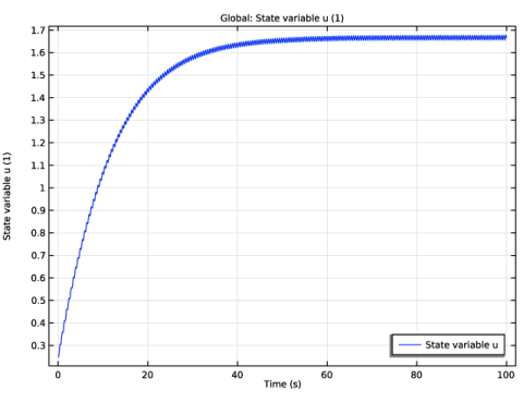
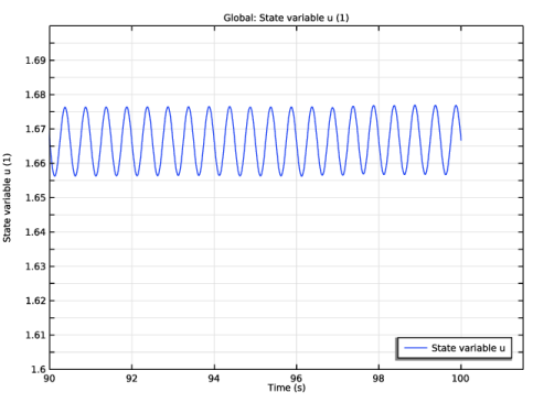
The time evolution of u is plotted in Figure 1. A close-up of the final few periods is plotted in Figure 2. This shows that u has indeed reached its periodic steady-state solution.
Figure 1: Plot of the evolution of u from its initial value of 0.25. There is a slow, steady increase in u over the first several periods along with oscillations at twice the driving frequency.
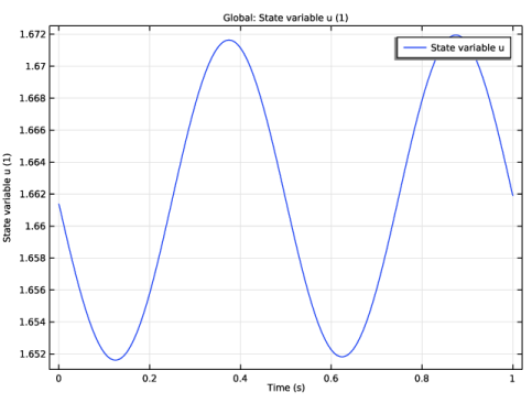
It is also obvious from Figure 2 that over 1 period, the value of u at the beginning of the period is the same as at the end of the period. In Figure 3 the solution computed by the optimization solver is shown. Note that the forward problem is only solved for 1 period. In total the optimization solver computes the solution to the forward problem only 6 times resulting in a much reduced simulation time.
Figure 2: Close up of the last several cycles of the forward problem. The model has clearly reached its periodic steady state solution after 100 cycles.
Figure 3: Plot of the solution computed by the optimization solver.
Reference
1. D.P. Lymberopoulos and D.J. Economou, “Fluid simulation of glow discharges: Effect of metastable atoms in argon,” J. Appl. Phys. vol. 73, no. 8, 1993.
Application Library path: Optimization_Module/Parameter_Estimation/time_dependent_optimization
Modeling Instructions
From the File menu, choose New.
New
In the New window, click  Model Wizard.
Model Wizard
1
In the Model Wizard window, click  0D.
2
In the Select Physics tree, select Mathematics > ODE and DAE Interfaces > Global ODEs and DAEs (ge).
3
Click Add.
4
Click  Study.
5
In the Select Study tree, select General Studies > Time Dependent.
6
Global Definitions
Parameters 1
1
In the Model Builder window, under Global Definitions click Parameters 1.
2
In the Settings window for Parameters, locate the Parameters section.
3
Global ODEs and DAEs (ge)
Define the ordinary differential equation with the periodic forcing function.
Global Equations 1 (ODE1)
1
In the Model Builder window, under Component 1 (comp1) > Global ODEs and DAEs (ge) click Global Equations 1 (ODE1).
2
In the Settings window for Global Equations, locate the Global Equations section.
3
Study 1
The model needs to be solved for 100 periods before it reaches its periodic steady state solution.
Step 1: Time Dependent
1
In the Model Builder window, under Study 1 click Step 1: Time Dependent.
2
In the Settings window for Time Dependent, locate the Study Settings section.
3
From the Tolerance list, choose User controlled.
4
In the Relative tolerance text field, type 1e-5.
5
In the Output times text field, type range(0,0.01,100).
Solution 1 (sol1)
1
In the Study toolbar, click  Show Default Solver.
2
In the Model Builder window, expand the Solution 1 (sol1) node, then click Time-Dependent Solver 1.
3
In the Settings window for Time-Dependent Solver, click to expand the Absolute Tolerance section.
4
From the Tolerance method list, choose Manual.
5
In the Absolute tolerance text field, type 0.0001.
6
In the Study toolbar, click  Compute.
Results
1D Plot Group 1
1
In the Settings window for 1D Plot Group, locate the Legend section.
2
From the Position list, choose Lower right.
3
In the 1D Plot Group 1 toolbar, click  Plot.
1D Plot Group 2
1
Right-click Results > 1D Plot Group 1 and choose Duplicate.
2
In the Settings window for 1D Plot Group, locate the Axis section.
3
Select the Manual axis limits checkbox.
4
In the x minimum text field, type 90.
5
In the y minimum text field, type 1.6.
6
In the y maximum text field, type 1.7.
7
In the 1D Plot Group 2 toolbar, click  Plot.
Root
Now add another study with an Optimization step which can be used to immediately compute the periodic steady state solution for the differential equation.
Add Study
1
In the Home toolbar, click  Add Study to open the Add Study window.
2
Go to the Add Study window.
3
Find the Studies subsection. In the Select Study tree, select General Studies > Time Dependent.
4
Click the Add Study button in the window toolbar.
5
In the Home toolbar, click  Add Study to close the Add Study window.
Study 2
Step 1: Time Dependent
1
In the Settings window for Time Dependent, locate the Study Settings section.
2
In the Output times text field, type range(0,0.002,1).
3
From the Tolerance list, choose User controlled.
4
In the Relative tolerance text field, type 1e-5.
General Optimization
1
In the Study toolbar, click  Optimization and choose General Optimization.
2
In the Settings window for General Optimization, locate the Optimization Solver section.
3
From the Method list, choose IPOPT.
Add the difference between initial and final value in a cycle as error measure to be minimized.
4
Locate the Objective Function section. In the table, enter the following settings:
Next, add the initial value as control parameter and set suitable bounds to help the solver.
5
Locate the Control Variables and Parameters section. Click  Add.
6
Solution 2 (sol2)
1
In the Study toolbar, click  Show Default Solver.
2
In the Model Builder window, expand the Solution 2 (sol2) node.
3
In the Model Builder window, expand the Study 2 > Solver Configurations > Solution 2 (sol2) > Optimization Solver 1 node, then click Time-Dependent Solver 1.
4
In the Settings window for Time-Dependent Solver, click to expand the Absolute Tolerance section.
5
From the Tolerance method list, choose Manual.
6
In the Absolute tolerance text field, type 1e-5.
7
In the Study toolbar, click  Compute.
The solver will issue a warning as a reminder that the objective function is only evaluated at the final time — which is indeed the desired behavior in this model.
Results
1D Plot Group 3
1
Click the  Zoom Extents button in the Graphics toolbar.
The periodic steady state solution is obtained (compare to Figure 2).