PDF

Neutralization of a Proton Beam Through a Charge Exchange Cell
Introduction
Collisions of neutral particle beams with target materials at various projectile energies are important in a number of applications ranging from plasma physics to material processing.
Beams of high-velocity neutral particles can be obtained using charge exchange cells. A charge exchange cell is a region of high-density gas placed on the path of an ion beam. The region of high gas density creates a medium in which fast ions can be neutralized to generate a beam of neutral particles at the exit of the cell.
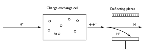
Figure 1 shows the concept behind a charge exchange cell. Protons are accelerated toward a cell filled with neutral argon. When they pass through the charge exchange cell, the protons can capture electrons from the argon atoms and exit the cell as fast neutral hydrogen atoms. Since the probability of electron capture is not very high, charged particles are still present in the beam as it exits the cell. In order to get a pure neutral beam at the end of the process, charged plates can be used to deflect the charged particles before the beam reaches its target.
This model uses the Molecular Flow Module to compute the pressure in the charge exchange cell. The Electrostatics interface is used to compute the electric field that deflects the charged particles. The Charged Particle Tracing interface is used to compute the trajectories and to simulate collisions between the particles and ambient neutral atoms.
Figure 1: Schematic of a simplified charge exchange cell neutralization process.
Model Definition
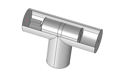
The geometry used in the model is shown in Figure 2. The gas cell consists of a tube 40 mm in diameter and 100 mm long. The tube has end caps with 2 mm diameter apertures along the cylinder axis. The argon gas is introduced into the gas cell through a shower head ring located in the center of the cell. The microchannels of the shower head are used to control the neutral gas density in the cell and create a high-pressure region within the main vacuum system of the instrument. To model the gas inflow the Outgassing Wall boundary condition is used. The gas cell is mounted in a vacuum “T”, which is pumped by a turbomolecular pump (pumping speed of 63 L/s).
The deflecting plates are modeled as two blocks. An electric potential of 200 V is applied on the upper plate while the lower plate is grounded.
As a first approximation, the charge exchange collisions are assumed to have a negligible effect on the direction of particle motion. The energies involved in the collisions are taken from Ref. 1 and are presented in the following reactions.
1: H+ + Ar -> H + Ar+, energy loss = 2.16 eV
2: H + Ar -> H+ + e + Ar, energy loss = 13.6 eV
Figure 2: Schematic of the model geometry.
Results and Discussion
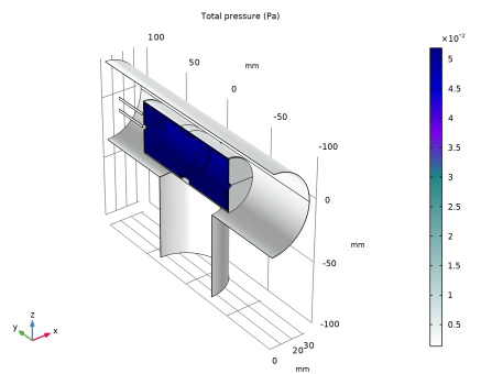
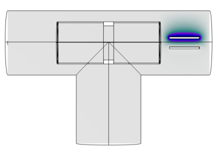
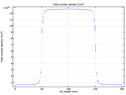
The electric potential distribution in the region surrounding the two plates is plotted in Figure 3. A surface plot of the pressure in the apparatus is shown in Figure 4. The corresponding number density is computed along the symmetry axis of the cylindrical cell and is plotted in Figure 5.
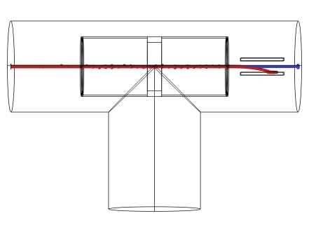
The particle trajectories are plotted in Figure 6. The color expression in this plot indicates the charge number of the atoms, which decreases from 1 (red) to 0 (blue) for particles that undergo charge exchange reactions in the cell. By comparing the number of particles on the plate to the total number of particles in the model, the neutralization efficiency is estimated to be 13.8%. Because the implementation of the charge exchange reactions is stochastic in nature, this value may change slightly when the model is re-run, depending on the seeding of random numbers.
Figure 3: Electric potential in the vacuum housing.
Figure 4: Pressure in the apparatus.
Figure 5: Axial number density through the gas cell and vacuum housing for argon for a constant mass flow rate of 0.05 sccm into the gas cell.
Figure 6: Particle trajectories. Ions are shown in red while neutrals are displayed in blue.
Reference
1. A. V. Phelps, “Collisions of H+, H2+, H3+, ArH+, H-, H, and H2 with Ar and of Ar+ and ArH+ with H2 for Energies from 0.1 eV to 10 keV,” J. Phys. Chem. Ref. Data, vol. 21, No. 4, pp. 883–897, 1992.
Application Library path: Molecular_Flow_Module/Industrial_Applications/charge_exchange_cell
Modeling Instructions
From the File menu, choose New.
New
In the New window, click  Model Wizard.
Model Wizard
1
In the Model Wizard window, click  3D.
2
In the Select Physics tree, select Fluid Flow > Rarefied Flow > Free Molecular Flow (fmf).
3
Click Add.
4
In the Select Physics tree, select AC/DC > Electric Fields and Currents > Electrostatics (es).
5
Click Add.
6
In the Select Physics tree, select AC/DC > Particle Tracing > Charged Particle Tracing (cpt).
7
Click Add.
8
Global Definitions
Parameters 1
Load the model parameters from a file.
1
In the Model Builder window, under Global Definitions click Parameters 1.
2
In the Settings window for Parameters, locate the Parameters section.
3
Click  Load from File.
4
Definitions
Enter raw data from Ref. 1 for the cross sections as a function of the primary particle energy.
Ar+H+=>H+Ar+
1
In the Definitions toolbar, click  Interpolation.
2
In the Settings window for Interpolation, type Ar+H+=>H+Ar+ in the Label text field.
3
Locate the Definition section. From the Data source list, choose File.
4
Click  Browse.
5
6
Click  Import.
7
In the Function name text field, type Qex1.
8
Locate the Units section. In the Argument table, enter the following settings:
9
In the Function table, enter the following settings:
H+Ar=>Ar+H+
1
In the Definitions toolbar, click  Interpolation.
2
In the Settings window for Interpolation, type H+Ar=>Ar+H+ in the Label text field.
3
Locate the Definition section. From the Data source list, choose File.
4
Click  Browse.
5
6
Click  Import.
7
In the Function name text field, type Qex2.
8
Locate the Units section. In the Argument table, enter the following settings:
9
In the Function table, enter the following settings:
H+Ar=>H+Ar+
1
In the Definitions toolbar, click  Interpolation.
2
In the Settings window for Interpolation, type H+Ar=>H+Ar+ in the Label text field.
3
Locate the Definition section. From the Data source list, choose File.
4
Click  Browse.
5
6
Click  Import.
7
In the Function name text field, type Qex3.
8
Locate the Units section. In the Argument table, enter the following settings:
9
In the Function table, enter the following settings:
Geometry 1
Insert the prepared geometry sequence from file. You can read the instructions for creating the geometry in the appendix.
1
In the Geometry toolbar, click Insert Sequence and choose Insert Sequence.
2
3
In the Geometry toolbar, click  Build All.
4
Click the  Wireframe Rendering button in the Graphics toolbar in order to see inside the geometry more easily.
Free Molecular Flow (fmf)
Set up the molecular flow simulation. Begin by entering the gas molar mass.
Molecular Flow 1
1
In the Model Builder window, under Component 1 (comp1) > Free Molecular Flow (fmf) click Molecular Flow 1.
2
In the Settings window for Molecular Flow, locate the Molecular Weight of Species section.
3
In the Mn,G text field, type M_gas.
Wall 2
1
In the Physics toolbar, click  Boundaries and choose Wall.
2
In the Settings window for Wall, locate the Wall Type section.
3
From the Wall type list, choose Outgassing wall.
4
Locate the Flux section. From the Outgoing flux list, choose Number of SCCM units.
5
In the Qsccm,G text field, type 0.05.
6
From the Standard flow rate defined by list, choose Standard pressure and temperature.
7
Vacuum Pump 1
Add the turbomolecular pump inlet.
1
In the Physics toolbar, click  Boundaries and choose Vacuum Pump.
2
3
In the Settings window for Vacuum Pump, locate the Vacuum Pump section.
4
From the Specify pump flux list, choose Pump speed.
5
In the SG text field, type 63[l/s].
In order to have a fast access to the number density in the apparatus, add a Number Density Reconstruction node.
Number Density Reconstruction 1
1
In the Physics toolbar, click  Domains and choose Number Density Reconstruction.
2
Electrostatics (es)
Now set up the electric field that will deflect the ions.
In the Model Builder window, under Component 1 (comp1) click Electrostatics (es).
Electric Potential 1
1
In the Physics toolbar, click  Boundaries and choose Electric Potential.
2
In the Settings window for Electric Potential, locate the Electric Potential section.
3
In the V0 text field, type 200[V].
4
Ground 1
1
In the Physics toolbar, click  Boundaries and choose Ground.
2
Alternatively, you could select all boundaries and then deselect only boundaries 41, 42, 43, 44, 46, 47, and 90, which are the faces of the upper block. A third option is to drag the Electric Potential 1 node below this node in the Model Builder, since these boundary conditions override each other.
Charged Particle Tracing (cpt)
1
In the Model Builder window, under Component 1 (comp1) click Charged Particle Tracing (cpt).
2
In the Settings window for Charged Particle Tracing, locate the Particle Release and Propagation section.
3
In the Maximum number of secondary particles text field, type 500.
H+
1
In the Model Builder window, under Component 1 (comp1) > Charged Particle Tracing (cpt) click Particle Properties 1.
2
In the Settings window for Particle Properties, type H+ in the Label text field.
3
Locate the Particle Mass section. In the mp text field, type M_p/N_A_const.
4
Locate the Charge Number section. In the Z text field, type 1.
H
1
In the Physics toolbar, click  Global and choose Particle Properties.
2
In the Settings window for Particle Properties, locate the Particle Mass section.
3
In the mp text field, type M_p/N_A_const.
4
Locate the Charge Number section. In the Z text field, type 0.
5
In the Label text field, type H.
Ar+
1
In the Physics toolbar, click  Global and choose Particle Properties.
2
In the Settings window for Particle Properties, type Ar+ in the Label text field.
3
Locate the Particle Mass section. In the mp text field, type M_gas/N_A_const.
4
Locate the Charge Number section. In the Z text field, type 1.
Particle Beam 1
1
In the Physics toolbar, click  Boundaries and choose Particle Beam.
2
3
In the Settings window for Particle Beam, locate the Initial Position section.
4
In the N text field, type N0.
5
Locate the Initial Transverse Velocity section. In the εrms text field, type 0.1[um].
6
Locate the Initial Longitudinal Velocity section. In the E text field, type 1[keV].
Electric Force 1
1
In the Physics toolbar, click  Domains and choose Electric Force.
2
3
In the Settings window for Electric Force, locate the Electric Force section.
4
From the E list, choose Electric field (es/fsp1).
Ar+H+=>H+Ar+
1
In the Physics toolbar, click  Domains and choose Collisions.
2
In the Settings window for Collisions, type Ar+H+=>H+Ar+ in the Label text field.
3
4
Locate the Fluid Properties section. In the Nd text field, type fmf.n_G.
5
Locate the Affected Particles section. From the Particles to affect list, choose Single species.
Nonresonant Charge Exchange 1
1
In the Physics toolbar, click  Attributes and choose Nonresonant Charge Exchange.
2
In the Settings window for Nonresonant Charge Exchange, locate the Collision Frequency section.
3
In the σ text field, type Qex1(cpt.Ep).
4
In the ΔE text field, type E1.
5
From the Species to release list, choose Ion and neutral particle.
6
Click to expand the Ion Properties section. From the Ion properties list, choose Ar+.
7
Click to expand the Neutral Properties section. From the Neutral properties list, choose H.
8
Locate the Collision Statistics section. Select the Count collisions checkbox.
H+Ar=>Ar+H+
1
In the Model Builder window, right-click Ar+H+=>H+Ar+ and choose Duplicate.
2
In the Settings window for Collisions, type H+Ar=>Ar+H+ in the Label text field.
3
Locate the Affected Particles section. From the Affected particle properties list, choose H.
Nonresonant Charge Exchange 1
1
In the Model Builder window, expand the H+Ar=>Ar+H+ node, then click Nonresonant Charge Exchange 1.
2
In the Settings window for Nonresonant Charge Exchange, locate the Collision Frequency section.
3
In the σ text field, type Qex2(cpt.Ep).
4
In the ΔE text field, type E2.
5
From the Species to release list, choose Ion.
6
Locate the Ion Properties section. From the Ion properties list, choose H+.
H+Ar=>H+Ar+
1
In the Model Builder window, right-click H+Ar=>Ar+H+ and choose Duplicate.
2
In the Settings window for Collisions, type H+Ar=>H+Ar+ in the Label text field.
Nonresonant Charge Exchange 1
1
In the Model Builder window, expand the H+Ar=>H+Ar+ node, then click Nonresonant Charge Exchange 1.
2
In the Settings window for Nonresonant Charge Exchange, locate the Collision Frequency section.
3
In the σ text field, type Qex3(cpt.Ep).
4
In the ΔE text field, type E3.
5
Locate the Ion Properties section. From the Ion properties list, choose Ar+.
For postprocessing purposes, create variables for collision statistics.
Definitions
Variables 1
1
In the Model Builder window, under Component 1 (comp1) right-click Definitions and choose Variables.
2
In the Settings window for Variables, locate the Variables section.
3
For postprocessing purposes, create a box selection.
Box 1
1
In the Definitions toolbar, click  Box.
2
In the Settings window for Box, locate the Box Limits section.
3
In the x minimum text field, type 0.
4
Locate the Geometric Entity Level section. From the Level list, choose Boundary.
5
Locate the Output Entities section. From the Include entity if list, choose All vertices inside box.
Mesh 1
In the Model Builder window, under Component 1 (comp1) right-click Mesh 1 and choose Edit Physics-Induced Sequence.
Size 3
1
In the Model Builder window, under Component 1 (comp1) > Mesh 1 right-click Size 3 and choose Disable.
2
In the Settings window for Size, click  Build All.
Root
Add a stationary study to compute the gas number density and electric field in the vacuum housing and charge exchange cell.
Add Study
1
In the Home toolbar, click  Add Study to open the Add Study window.
2
Go to the Add Study window.
3
Find the Physics interfaces in study subsection. In the table, clear the Solve checkbox for Charged Particle Tracing (cpt).
4
Find the Studies subsection. In the Select Study tree, select General Studies > Stationary.
5
Click the Add Study button in the window toolbar.
6
In the Home toolbar, click  Add Study to close the Add Study window.
Study 1
Solution 1 (sol1)
1
In the Study toolbar, click  Show Default Solver.
2
In the Model Builder window, expand the Solution 1 (sol1) node.
3
In the Model Builder window, expand the Study 1 > Solver Configurations > Solution 1 (sol1) > Stationary Solver 1 > Iterative 2 node, then click Multigrid 1.
4
In the Settings window for Multigrid, locate the General section.
5
In the Mesh coarsening factor text field, type 1.
6
In the Model Builder window, click Study 1.
7
In the Settings window for Study, locate the Study Settings section.
8
Clear the Generate default plots checkbox.
9
In the Study toolbar, click  Compute.
Create a new dataset using the Box 1 selection that was defined earlier.
Results
In the Model Builder window, expand the Results node.
Study 1/Solution 1 Box Selection
1
In the Model Builder window, expand the Results > Datasets node.
2
Right-click Results > Datasets > Study 1/Solution 1 (sol1) and choose Duplicate.
3
In the Settings window for Solution, type Study 1/Solution 1 Box Selection in the Label text field.
Selection
1
In the Results toolbar, click  Attributes and choose Selection.
2
In the Settings window for Selection, locate the Geometric Entity Selection section.
3
From the Geometric entity level list, choose Boundary.
4
From the Selection list, choose Box 1.
Create a Cut Line dataset along the beam line center.
Cut Line 3D 1
1
In the Results toolbar, click  Cut Line 3D.
2
In the Settings window for Cut Line 3D, locate the Line Data section.
3
In row Point 1, set y to -100.
4
In row Point 2, set y to 100 and x to 0.
Plot the electric potential created by the deflecting plates.
Electric Potential
1
In the Results toolbar, click  3D Plot Group.
2
In the Settings window for 3D Plot Group, type Electric Potential in the Label text field.
Slice 1
1
Right-click Electric Potential and choose Slice.
2
In the Settings window for Slice, locate the Plane Data section.
3
In the Planes text field, type 1.
4
Click the  Go to YZ View button in the Graphics toolbar.
5
Locate the Expression section. In the Expression text field, type V.
6
Locate the Coloring and Style section. From the Color table list, choose AuroraAustralis.
7
In the Electric Potential toolbar, click  Plot.
8
Click the  Zoom Extents button in the Graphics toolbar.
Plot the pressure in the apparatus.
Pressure
1
In the Results toolbar, click  3D Plot Group.
2
In the Settings window for 3D Plot Group, type Pressure in the Label text field.
3
Locate the Data section. From the Dataset list, choose Study 1/Solution 1 Box Selection (sol1).
Surface 1
1
Right-click Pressure and choose Surface.
2
In the Settings window for Surface, locate the Expression section.
3
In the Expression text field, type fmf.ptot.
4
Locate the Coloring and Style section. From the Color table list, choose AuroraAustralis.
5
In the Pressure toolbar, click  Plot.
6
Click the  Go to Default View button in the Graphics toolbar.
Plot the neutral gas number density along the center of the beam line.
Gas Number Density
1
In the Results toolbar, click  1D Plot Group.
2
In the Settings window for 1D Plot Group, type Gas Number Density in the Label text field.
3
Locate the Data section. From the Dataset list, choose Cut Line 3D 1.
Line Graph 1
1
Right-click Gas Number Density and choose Line Graph.
2
In the Settings window for Line Graph, locate the y-Axis Data section.
3
In the Expression text field, type fmf.ntot.
4
In the Gas Number Density toolbar, click  Plot.
Add a transient study to simulate the beam neutralization.
Add Study
1
In the Home toolbar, click  Add Study to open the Add Study window.
2
Go to the Add Study window.
3
Find the Physics interfaces in study subsection. In the table, clear the Solve checkboxes for Free Molecular Flow (fmf) and Electrostatics (es).
4
Find the Studies subsection. In the Select Study tree, select General Studies > Time Dependent.
5
Click the Add Study button in the window toolbar.
6
In the Home toolbar, click  Add Study to close the Add Study window.
Study 2
Step 1: Time Dependent
Use the values of variables computed from the previous study, that is, the electric field and the gas number density.
1
In the Settings window for Time Dependent, locate the Study Settings section.
2
From the Time unit list, choose µs.
3
Click  Range.
4
In the Range dialog, type 0.01 in the Step text field.
5
In the Stop text field, type 0.5.
6
Click Replace.
7
In the Settings window for Time Dependent, click to expand the Values of Dependent Variables section.
8
Find the Values of variables not solved for subsection. From the Settings list, choose User controlled.
9
From the Method list, choose Solution.
10
From the Study list, choose Study 1, Stationary.
Set the maximum time step taken by the solver to be about an order of magnitude less than the inverse of the collision frequency. This is an important detail for the Monte Carlo collision model because collisions are only applied at discrete time steps taken by the solver.
Solution 2 (sol2)
1
In the Study toolbar, click  Show Default Solver.
2
In the Model Builder window, expand the Solution 2 (sol2) node, then click Time-Dependent Solver 1.
3
In the Settings window for Time-Dependent Solver, click to expand the Time Stepping section.
4
From the Maximum step constraint list, choose Constant.
5
In the Maximum step text field, type 10[ns].
Step 1: Time Dependent
In the Study toolbar, click  Compute.
Results
Particle Trajectories (cpt)
A default Particle Trajectories plot is created. Display the particle charge in the Color Expression 1 subnode.
Particle Trajectories 1
1
In the Model Builder window, expand the Particle Trajectories (cpt) node, then click Particle Trajectories 1.
2
In the Settings window for Particle Trajectories, locate the Coloring and Style section.
3
Find the Line style subsection. From the Type list, choose Line.
Color Expression 1
1
In the Model Builder window, expand the Particle Trajectories 1 node, then click Color Expression 1.
2
In the Settings window for Color Expression, locate the Expression section.
3
In the Expression text field, type cpt.Z.
4
Locate the Coloring and Style section. From the Color table list, choose RainbowLight.
5
Click the  Go to YZ View button in the Graphics toolbar.
6
In the Particle Trajectories (cpt) toolbar, click  Plot.
7
Click the  Zoom Extents button in the Graphics toolbar.
Compute the neutralization efficiency. Duplicate the Particle 1 dataset and create a boundary selection for the wall at the opposite of the aperture wall.
Particle 2
In the Model Builder window, under Results > Datasets right-click Particle 1 and choose Duplicate.
Selection
1
In the Results toolbar, click  Attributes and choose Selection.
2
In the Settings window for Selection, locate the Geometric Entity Selection section.
3
From the Geometric entity level list, choose Boundary.
4
Efficiency
1
In the Results toolbar, click  Global Evaluation.
2
In the Settings window for Global Evaluation, type Efficiency in the Label text field.
3
Locate the Data section. From the Dataset list, choose Particle 2.
4
From the Time selection list, choose Last.
5
Locate the Expressions section. In the table, enter the following settings:
Nc1/Nctot
1
Right-click Efficiency and choose Duplicate.
2
In the Settings window for Global Evaluation, type Nc1/Nctot in the Label text field.
3
Locate the Expressions section. In the table, enter the following settings:
Nc2/Nctot
1
Right-click Nc1/Nctot and choose Duplicate.
2
In the Settings window for Global Evaluation, type Nc2/Nctot in the Label text field.
3
Locate the Expressions section. In the table, enter the following settings:
Nc3/Nctot
1
Right-click Nc2/Nctot and choose Duplicate.
2
In the Settings window for Global Evaluation, type Nc3/Nctot in the Label text field.
3
Locate the Expressions section. In the table, enter the following settings:
4
In the Results toolbar, click  Evaluate and choose Clear and Evaluate All.
Table 4
Go to the Table 4 window. Results are displayed in tables 1 to 4 by clicking on the associated node under the Derived Values node.
Appendix — Geometry Instructions
Geometry 1
1
In the Model Builder window, under Component 1 (comp1) click Geometry 1.
2
In the Settings window for Geometry, locate the Units section.
3
From the Length unit list, choose mm.
The gas cell geometry is created by filling in a cross section and then taking the solid of revolution.
Work Plane 1 (wp1)
1
In the Geometry toolbar, click  Work Plane.
2
In the Settings window for Work Plane, locate the Unite Objects section.
3
Clear the Unite objects checkbox.
4
Click  Go to Plane Geometry.
Work Plane 1 (wp1) > Rectangle 1 (r1)
1
In the Work Plane toolbar, click  Rectangle.
2
In the Settings window for Rectangle, locate the Size and Shape section.
3
In the Width text field, type 4.
4
In the Height text field, type 10.
5
Locate the Position section. In the xw text field, type 17.
6
In the yw text field, type -5.
Work Plane 1 (wp1) > Rectangle 2 (r2)
1
In the Work Plane toolbar, click  Rectangle.
2
In the Settings window for Rectangle, locate the Size and Shape section.
3
In the Height text field, type 100.
4
Locate the Position section. In the xw text field, type 20.
5
In the yw text field, type -50.
Work Plane 1 (wp1) > Rectangle 3 (r3)
1
In the Work Plane toolbar, click  Rectangle.
2
In the Settings window for Rectangle, locate the Size and Shape section.
3
In the Width text field, type 19.
4
Locate the Position section. In the xw text field, type 2.
5
In the yw text field, type 50.
Work Plane 1 (wp1) > Rectangle 4 (r4)
1
In the Work Plane toolbar, click  Rectangle.
2
In the Settings window for Rectangle, locate the Size and Shape section.
3
In the Width text field, type 19.
4
Locate the Position section. In the xw text field, type 2.
5
In the yw text field, type -51.
6
Click the  Zoom Extents button in the Graphics toolbar.
Work Plane 1 (wp1) > Union 1 (uni1)
1
In the Work Plane toolbar, click  Booleans and Partitions and choose Union.
2
Click in the Graphics window and then press Ctrl+A to select all objects.
3
In the Settings window for Union, click  Build Selected.
Revolve 1 (rev1)
1
In the Model Builder window, right-click Geometry 1 and choose Revolve.
2
In the Settings window for Revolve, click  Build Selected.
Create the vacuum housing that surrounds the gas cell.
Cylinder 1 (cyl1)
1
In the Geometry toolbar, click  Cylinder.
2
In the Settings window for Cylinder, locate the Size and Shape section.
3
In the Radius text field, type 32.
4
In the Height text field, type 200.
5
Locate the Position section. In the y text field, type -100.
6
Locate the Axis section. From the Axis type list, choose y-axis.
Cylinder 2 (cyl2)
1
In the Geometry toolbar, click  Cylinder.
2
In the Settings window for Cylinder, locate the Size and Shape section.
3
In the Radius text field, type 32.
4
In the Height text field, type 100.
5
Locate the Position section. In the z text field, type -100.
6
Click  Build Selected.
7
Click the  Zoom Extents button in the Graphics toolbar.
Union 1 (uni1)
1
In the Geometry toolbar, click  Booleans and Partitions and choose Union.
2
Select the objects cyl1 and cyl2 only.
3
In the Settings window for Union, locate the Union section.
4
Clear the Keep interior boundaries checkbox.
5
Click  Build Selected.
Create two blocks to represent the deflecting plates.
Block 1 (blk1)
1
In the Geometry toolbar, click  Block.
2
In the Settings window for Block, locate the Size and Shape section.
3
In the Width text field, type 10.
4
In the Depth text field, type 30.
5
In the Height text field, type 2.
6
Locate the Position section. From the Base list, choose Center.
7
In the y text field, type 75.
8
In the z text field, type 5.
Block 2 (blk2)
1
In the Geometry toolbar, click  Block.
2
In the Settings window for Block, locate the Size and Shape section.
3
In the Width text field, type 10.
4
In the Depth text field, type 30.
5
In the Height text field, type 2.
6
Locate the Position section. From the Base list, choose Center.
7
In the y text field, type 75.
8
In the z text field, type -5.
9
Click  Build Selected.
Subtract all solid domains from the geometry. The simulation domain is just the volume within the gas cell and vacuum chamber, where the beam will propagate.
Difference 1 (dif1)
1
In the Geometry toolbar, click  Booleans and Partitions and choose Difference.
2
3
In the Settings window for Difference, locate the Difference section.
4
Click to select the  Activate Selection toggle button for Objects to subtract.
5
Select the objects blk1, blk2, and rev1 only.
6
Click  Build Selected.
Create an aperture for the ion beam to enter on one side of the chamber.
Work Plane 2 (wp2)
1
In the Geometry toolbar, click  Work Plane.
2
In the Settings window for Work Plane, locate the Plane Definition section.
3
From the Plane list, choose xz-plane.
4
In the y-coordinate text field, type -100.
5
Click  Go to Plane Geometry.
Work Plane 2 (wp2) > Circle 1 (c1)
1
In the Work Plane toolbar, click  Circle.
2
In the Settings window for Circle, locate the Size and Shape section.
3
In the Radius text field, type 2.
4
In the Work Plane toolbar, click  Build All.
5
Click the  Zoom Extents button in the Graphics toolbar.
6
Right-click Geometry 1 and choose Build All.
7
Click the  Zoom Extents button in the Graphics toolbar.