COMSOL 6.4 - Free Surface Mixer Level Set

This example of turbulent two-phase flow in a partially baffled mixer shows how to set up a time dependent, turbulent two-phase flow simulation together with a rotating domain. The interface between the two fluids, water and air, is modeled using a level-set approach, and turbulence is modeled using the k-ε turbulence model. The mixer geometry used in this model corresponds to the one used by J.-P. Torré and others (Ref. 1), and the results can be compared with experiments.

Model Definition

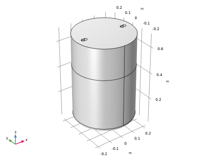
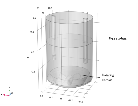
The mixer is a glass-lined, under-baffled stirred vessel. Figure 1 shows the model geometry. The mixer includes a three-bladed impeller and two beavertail baffles supported at the top of the vessel. The tank bottom is curved, allowing the three-bladed impeller to be placed close to the bottom. The cylindrical part of the tank has a diameter of 450 mm, and the initial water level is 467 mm. The two contoured baffles hang from the top of the mixer, and their lower part is 256 mm above the bottom of the vessel.

Figure 1: Geometry of the mixer with two rods and a three-bladed impeller.

The model uses a time dependent simulation starting from rest. The rotational velocity of the impeller is gradually increased until it reaches 275 rpm at t = 5 s, and the simulation is continued until t = 5.5 s. The flow in the mixer is modeled using a Two-Phase Flow, Level Set physics interface, to track the interface between water and air, with a k-ε turbulence model.

Results and Discussion

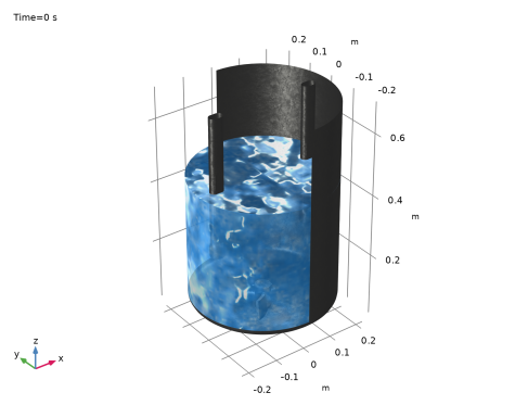
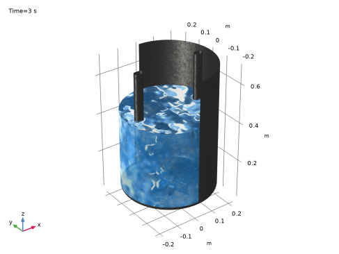
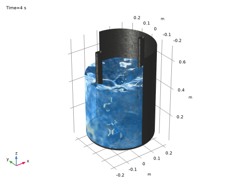
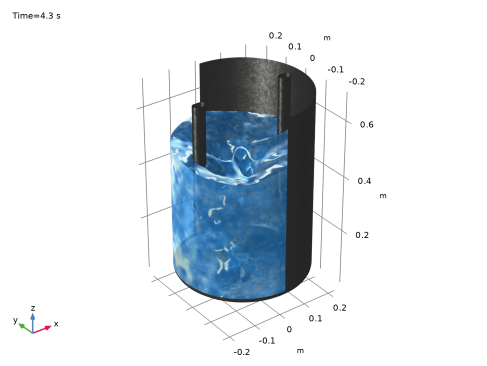
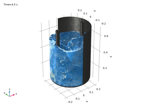
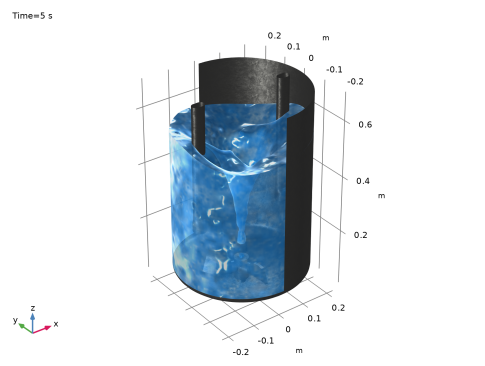
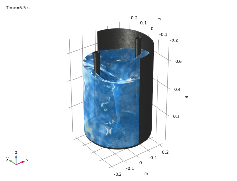
The results, presented in this section, focus on the shape of the unstable free surface. The free surface is plotted at different times in Figure 2 to Figure 8. The surface remains essentially unperturbed until, at around t = 4.0 s, it starts forming a “bath-tub vortex.” The vortex is fully developed and reaches the bottom at t = 4.5 s. Once the impeller reaches the maximum rotational velocity, at t = 5 s, the shape of the free surface agrees with the experimental and numerical results presented in Ref. 1. The vortex is more or less stable for a short while before it breaks at the impeller and air bubbles are entrained into the water bulk. This last stage is not included in this model, but can be observed if the simulation is extended for another second.

Figure 2: Water surface position at t = 0 s.

Figure 3: Water surface position at t = 3.0 s. The impeller is rotating at 187 rpm, but the rotation has not yet affected the shape of the free surface.

Figure 4: Water surface position at t = 4.0 s. The impeller is already rotating at 259 rpm, and the free surface has started to deform.

Figure 5: Water surface position at t = 4.3 s. The impeller is almost rotating at the maximum speed, and the free surface is forming a bath-tub vortex.

Figure 6: Water surface position at t = 4.5 s. The free surface has reached the impeller and the vortex remains semi-stable for about one second.

Figure 7: Water surface position at t = 5.0 s. The impeller has reached the maximum rotating velocity of 275 rpm. The vortex shape is fully developed and can be compared with experimental data.

Figure 8: Water surface position at t = 5.5 s. The mixer has been rotating at constant velocity for 0.5 s and the vortex remains more or less stable. Should the model be simulated for longer time, the vortex shape would break at the impeller and air bubbles would be shed away.

Notes About the COMSOL Implementation

The present application uses the Block-Navier–Stokes preconditioner instead of the default preconditioner for GMRES when solving the Navier–Stokes equations. This preconditioner can uncouple the pressure and velocity equations when solving, and may provide faster solutions for large time-dependent incompressible models with high Reynolds numbers or low viscosities.

Reference

1. J.-P. Torré and others, “An Experimental and Computational Study of the Vortex Shape in a Partially Baffled Agitated Vessel,” Chem. Eng. Sci., vol. 62, no. 7, pp. 1915–1926, 2007.

Mixer_Module/Tutorials/free_surface_mixer_ls

Modeling Instructions

From the menu, choose .

New

In the window, click

Model Wizard

In the window, click

In the tree, select > > > > ε.

Click .

Click

In the tree, select > .

Click

Geometry 1

As the main focus will be on the physics and numerics, a detailed treatment of the geometry building procedure lies outside the scope of this tutorial. Instead, the geometry has been prepared in the file free_surface_mixer_geom_sequence.mph. You can start by inserting the geometry sequence from that file.

In the toolbar, click and choose .

Browse to the model’s Application Libraries folder and double-click the file free_surface_mixer_geom_sequence.mph.

In the toolbar, click

In the window, under click .

Click the

button in the toolbar.

Click the

button in the toolbar.

Define a step function to be used when ramping up the rotational velocity.

Global Definitions

Step 1 (step1)

In the toolbar, click

and choose > .

In the window for , locate the section.

In the text field, type 2.5.

Click to expand the section. In the text field, type 5.

Moving Mesh

Rotating Domain 1

In the window, under > click .

In the window for , locate the section.

In the list, choose and .

Click

Select Domain 3 only.

Locate the section. In the f text field, type 275[rpm]*step1(t[1/s]).

Locate the section. Specify the urot vector as


0	X
0	Y
1	Z

Next, add a to compute effective material properties, and define phase from the Material Library.

Multiphysics

Two-Phase Flow, Level Set 1 (tpf1)

In the window, under > click .

In the window for , locate the section.

Click

Materials

Phase 1 (mpmat1.phase1)

In the window, under > > click .

In the window for , locate the section.

Click

. This button is found when expanding the options next to the list.

Add Material to Phase 1 (mpmat1.phase1)

Go to the window.

In the tree, select > .

Click .

Materials

Phase 2 (mpmat1.phase2)

In the window, under > > click .

In the window for , locate the section.

Click

. This button is found when expanding the options next to the list.

Add Material to Phase 2 (mpmat1.phase2)

Go to the window.

In the tree, select > .

Click .

Materials

Click the

button in the toolbar.

In the dialog, in the tree, select the checkbox for the node > .

Click .

Turbulent Flow, k-ε (spf)

In the window, under click ε.

In the window for ε, locate the section.

Select the checkbox.

Click to expand the section. Find the subsection. Select the checkbox. This preconditioner is efficient for time dependent incompressible flow problems.

Next, set up an initial pressure that accounts for the presence of both phases.

Initial Values 1

In the window, under > ε (spf) click .

In the window for , locate the section.

In the p text field, type tpf1.rho2*g_const*(0.7[m]-z)*ls.Vf2+tpf1.rho1*g_const*(0.4667[m]-z)*ls.Vf1.

Clear the checkbox.

Pressure Point Constraint 1

In the toolbar, click

and choose .

Select Point 22 only.

In the window for , locate the section.

Clear the checkbox.

Level Set (ls)

Initial Values, Fluid 2

In the window, under > click .

Select Domain 2 only.

Multiphysics

Wetted Wall, Automatic from frame

In the toolbar, click

and choose > .

In the window for , type Wetted Wall, Automatic from frame in the text field.

Locate the section. From the list, choose .

In the list box, select .

Click

The is set per default to . This means that the boundaries adjacent to the will rotate due to the angular velocity. However, boundary 32 (the base of the mixer) is adjacent to the but should not rotate. Add a new feature and set the to .

Wetted Wall, Fixed wall

In the toolbar, click