|
|
|

|
|
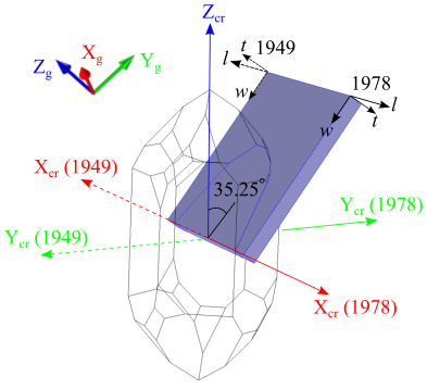
When defining the material properties of quartz, the orientation of the crystal axes X, Y, and Z with respect to the crystal differs between the 1978 IEEE standard and the 1949 IRE standard, as shown in Figure 3. (In the figure the crystal axes X, Y, and Z are labeled as Xcr, Ycr, and Zcr for clarity.) A consequence of this is that both the material property matrices and the crystal cut differ between the two standards. Table 1 summarizes the signs for the important matrix elements under the two conventions. Table 2 shows the different definitions of the crystal cuts under the two conventions.
|
|
1
|
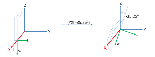
The IRE or IEEE standard defines the relationship between the crystal axes (Xcr, Ycr, Zcr) and the plate axes (l, w, t).
|
|
2
|
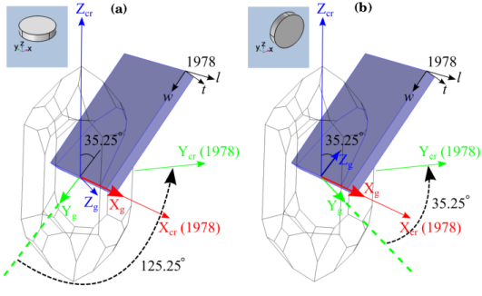
When creating a COMSOL Multiphysics model, we draw the plate in the geometry window, thereby implicitly defines the relationship between the plate axes (l, w, t) and the global axes (Xg, Yg, Zg). If the plate is oriented differently in the model geometry, then this relationship will also be different.
|
|
3
|
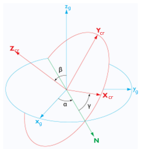
Using the two relationships above, we can determine the relationship between the crystal axes (Xcr, Ycr, and Zcr) and the global axes (Xg, Yg, and Zg).
|
|
1
|
|
2
|
In the Select Physics tree, select Structural Mechanics > Electromagnetics–Structure Interaction > Piezoelectricity > Piezoelectricity, Solid.
|
|
3
|
Click Add.
|
|
4
|
Click
|
|
1
|
|
2
|
|
1
|
|
2
|
|
3
|
Click
|
|
4
|
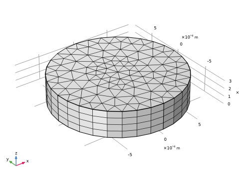
Browse to the model’s Application Libraries folder and double-click the file thickness_shear_quartz_oscillator_mesh.mphbin.
|
|
5
|
Click
|
|
1
|
|
2
|
|
3
|
|
1
|
|
2
|
|
3
|
|
4
|
Select the All boundaries checkbox.
|
|
1
|
|
2
|
|
3
|
|
1
|
|
2
|
Go to the Add Material window.
|
|
3
|
|
4
|
Click the Add to Component button in the window toolbar.
|
|
5
|
|
1
|
In the Model Builder window, under Component 1 (comp1) > Solid Mechanics (solid) click Piezoelectric Material 1.
|
|
2
|
|
3
|
|
1
|
|
2
|
|
3
|
|
4
|
|
1
|
|
1
|
|
3
|
|
4
|
|
1
|
|
2
|
|
3
|
|
5
|
|
6
|
|
1
|
|
1
|
|
2
|
Go to the Add Physics window.
|
|
3
|
|
4
|
Click the Add to Component 1 button in the window toolbar.
|
|
5
|
|
1
|
|
2
|
|
4
|
|
5
|
|
1
|
|
2
|
|
4
|
|
1
|
|
2
|
|
3
|
|
4
|
|
1
|
|
1
|
|
2
|
Go to the Add Study window.
|
|
3
|
|
4
|
Click the Add Study button in the window toolbar.
|
|
5
|
|
1
|
In the Study toolbar, click
|
|
2
|
|
3
|
|
4
|
|
6
|
Locate the Physics and Variables Selection section. In the Solve for column of the table, under Component 1 (comp1), clear the checkbox for Electrical Circuit (cir).
|
|
7
|
|
1
|
|
2
|
|
3
|
|
1
|
|
2
|
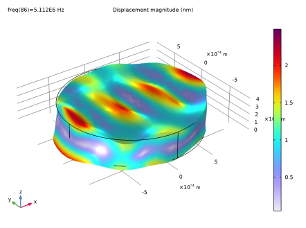
In the Settings window for Volume, click Replace Expression in the upper-right corner of the Expression section. From the menu, choose Component 1 (comp1) > Solid Mechanics > Displacement > solid.disp - Displacement magnitude - m.
|
|
3
|
|
4
|
|
5
|
|
1
|
|
2
|
|
3
|
|
1
|
|
2
|
|
3
|
|
4
|
|
5
|
|
6
|
|
7
|
|
8
|
|
1
|
|
2
|
|
3
|
|
4
|
|
5
|
|
6
|
|
7
|
|
8
|
|
9
|
|
1
|
|
2
|
|
1
|
|
3
|
|
4
|
|
5
|
|
6
|
|
7
|
|
1
|
|
2
|
Go to the Add Study window.
|
|
3
|
|
4
|
Click the Add Study button in the window toolbar.
|
|
5
|
|
1
|
In the Study toolbar, click
|
|
2
|
|
3
|
|
4
|
|
6
|
Locate the Physics and Variables Selection section. Select the Modify model configuration for study step checkbox.
|
|
7
|
|
8
|
Click
|
|
9
|
Click to expand the Store in Output section. In the table, enter the following settings:
|
|
10
|
|
11
|
|
12
|
Click OK.
|
|
13
|
|
15
|
|
16
|
|
17
|
Click OK.
|
|
1
|
|
2
|
|
3
|
Click
|
|
5
|
|
6
|
|
7
|
Clear the Generate default plots checkbox.
|
|
8
|
|
1
|
|
2
|
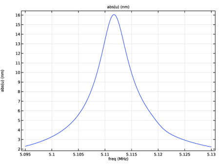
In the Settings window for 1D Plot Group, type Mechanical response, Parametric in the Label text field.
|
|
3
|
|
4
|
|
1
|
In the Model Builder window, expand the Mechanical response, Parametric node, then click Point Graph 1.
|
|
2
|
|
3
|
Select the Show legends checkbox.
|
|
4
|