PDF

Thermal Contact Resistance Between an Electronic Package and a Heat Sink
Introduction
This example reproduces parts of the study of Ref. 1 on the thermal contact resistance at the interface between a heat sink and an electronic package. As shown in Figure 1, eight cooling fins equip the cylindrical heat sink and contact is made at the radial boundaries of the package.
Figure 1: Heat sink with cooling fins around a cylindrical package.
The efficiency of the device depends on the cooling of the fins and the heat transfer from the package to the heat sink. This application focuses on the heat transfer through the contact interface where four parameters influence the joint conductance: contact pressure, microhardness of the softer material, surface roughness, and surface roughness slope.
Model Definition
The electronic package is simplified into a cylinder with radius 1 cm and height 5 cm and is made of silicon. The aluminum heat sink contains eight fins reaching a distance of 2 cm from the cylinder axis. Only 1/16th of the geometry is represented thanks to the symmetries shown in Figure 2.
Figure 2: Symmetry and simplification of the geometry.
The package produces a total heat source of 5 W. To dissipate it, air at 293.15 K and 1 atm resulting from a cooling fan, cools the heat sink fins by forced convection. The COMSOL Multiphysics built-in local heat transfer coefficient is used, assuming that the velocity of air is 8.5 m/s. The extremities of the device are thermally insulated.
At the contact interface, the thermal contact conductance h is expressed by (Ref. 1):
where the contact pressure, p, the aluminum microhardness, Hmic, the surface roughness, σ, and the roughness slope, m, are the four parameters studied here by a parametric sweep. Table 1 describes the quantities involved in these relations and gives the values (Ref. 1) used in the reference case.
The reference case uses the following additional relation for p ⁄ Hmic (4.16 in Ref. 2):
where c1, c2, and σ0 are detailed in Table 1.
Hmic
μm
ks
kgap
Mgap
c1
c2
Results and Discussion
Figure 3 shows the temperature profile obtained with the reference values. Near the fan, the temperature of the fins are about 483 K. It increases to reach 489 K at the opposite extremity.
Figure 3: Temperature profile with reference values for the parameters.
Figure 4 and Figure 5 plot the evolution of the constriction resistance according to p and Hmic and to σ and m. Figure 6 and Figure 7 display the analogous results for the gap resistance.
The contour curves are the same as in Ref. 1. Because the study in Ref. 1 is not in 3D but simplified into a 2D model, the values of contact resistance differ slightly. The last figure shows almost constant values in the vertical direction, meaning that m has little influence on the gap conductance.
Figure 4: Constriction resistance depending on contact pressure (x-axis) and microhardness (y-axis).
Figure 5: Constriction resistance depending on roughness (x-axis) and roughness slope (y-axis).
Figure 6: Gap resistance depending on contact pressure (x-axis) and microhardness (y-axis).
Figure 7: Gap resistance depending on roughness (x-axis) and roughness slope (y-axis).
References
1. M. Grujicic, C.L. Zhao, and E.C. Dusel, “The Effect of Thermal Resistance on Heat Management in the Electronic Packaging,” Applied Surface Science, vol. 246, pp. 290–302, 2005.
2. A. Bejan and A. D. Kraus, eds., Heat Transfer Handbook, John Wiley & Sons, 2003.
Application Library path: Heat_Transfer_Module/Thermal_Contact_and_Friction/thermal_contact_electronic_package_heat_sink
Modeling Instructions
From the File menu, choose New.
New
In the New window, click  Model Wizard.
Model Wizard
1
In the Model Wizard window, click  3D.
2
In the Select Physics tree, select Heat Transfer > Heat Transfer in Solids (ht).
3
Click Add.
4
Click  Study.
5
In the Select Study tree, select General Studies > Stationary.
6
Global Definitions
Parameters 1
1
In the Model Builder window, under Global Definitions click Parameters 1.
2
In the Settings window for Parameters, locate the Parameters section.
3
Geometry 1
Only 1/16th of the geometry is represented due to symmetry considerations in the device.
Work Plane 1 (wp1)
1
In the Geometry toolbar, click  Work Plane.
2
In the Settings window for Work Plane, locate the Plane Definition section.
3
From the Plane list, choose yz-plane.
4
Click  Go to Plane Geometry.
Work Plane 1 (wp1) > Circle 1 (c1)
1
In the Work Plane toolbar, click  Circle.
2
In the Settings window for Circle, locate the Size and Shape section.
3
In the Radius text field, type 2[cm].
4
In the Sector angle text field, type 360/16.
5
Click to expand the Layers section. In the table, enter the following settings:
6
Click  Build Selected.
Work Plane 1 (wp1) > Quadratic Bézier 1 (qb1)
1
In the Work Plane toolbar, click  More Primitives and choose Quadratic Bézier.
2
In the Settings window for Quadratic Bézier, locate the Control Points section.
3
In row 1, set xw to 2[cm], and yw to 0.6[cm].
4
In row 2, set xw to 0.4[cm].
5
In row 3, set xw to 2[cm], and yw to -0.6[cm].
Work Plane 1 (wp1) > Line Segment 1 (ls1)
1
In the Work Plane toolbar, click  More Primitives and choose Line Segment.
2
In the Settings window for Line Segment, locate the Starting Point section.
3
From the Specify list, choose Coordinates.
4
Locate the Endpoint section. From the Specify list, choose Coordinates.
5
Locate the Starting Point section. In the xw text field, type 2[cm].
6
In the yw text field, type 0.6[cm].
7
Locate the Endpoint section. In the xw text field, type 2[cm].
8
In the yw text field, type -0.6[cm].
Work Plane 1 (wp1) > Convert to Solid 1 (csol1)
1
In the Work Plane toolbar, click  Conversions and choose Convert to Solid.
2
Select the objects ls1 and qb1 only.
3
In the Settings window for Convert to Solid, click  Build Selected.
4
Click the  Zoom Extents button in the Graphics toolbar.
So far, the geometry should look like the figure below.
Work Plane 1 (wp1) > Partition Objects 1 (par1)
1
In the Work Plane toolbar, click  Booleans and Partitions and choose Partition Objects.
2
3
In the Settings window for Partition Objects, locate the Partition Objects section.
4
Click to select the  Activate Selection toggle button for Tool objects.
5
Work Plane 1 (wp1) > Delete Entities 1 (del1)
1
In the Model Builder window, right-click Plane Geometry and choose Delete Entities.
2
In the Settings window for Delete Entities, locate the Entities or Objects to Delete section.
3
From the Geometric entity level list, choose Domain.
4
On the object par1, select Domain 3 only.
5
Click  Build Selected.
Work Plane 1 (wp1)
1
In the Model Builder window, under Component 1 (comp1) > Geometry 1 click Work Plane 1 (wp1).
2
In the Settings window for Work Plane, click  Build Selected.
Extrude 1 (ext1)
1
In the Geometry toolbar, click  Extrude.
2
In the Settings window for Extrude, locate the Distances section.
3
4
In the Geometry toolbar, click  Build All.
5
Click the  Zoom Extents button in the Graphics toolbar.
Add Material
1
In the Materials toolbar, click  Add Material to open the Add Material window.
2
Go to the Add Material window.
3
In the tree, select Built-in > Aluminum.
4
Click the Add to Component button in the window toolbar.
5
In the tree, select Built-in > Silicon.
6
Click the Add to Component button in the window toolbar.
7
In the Materials toolbar, click  Add Material to close the Add Material window.
Materials
Silicon (mat2)
Select Domain 1 only.
Heat Transfer in Solids (ht)
Heat Source 1
1
In the Physics toolbar, click  Domains and choose Heat Source.
2
3
In the Settings window for Heat Source, locate the Heat Source section.
4
From the Heat source list, choose Heat rate.
5
In the P0 text field, type 5[W].
Heat Flux 1
1
In the Physics toolbar, click  Boundaries and choose Heat Flux.
2
3
In the Settings window for Heat Flux, locate the Heat Flux section.
4
From the Flux type list, choose Convective heat flux.
5
From the Heat transfer coefficient list, choose External forced convection.
6
From the list, choose Plate, local transfer coefficient.
7
In the xpl text field, type x.
8
In the U text field, type 8.5[m/s].
Thermal Contact 1
1
In the Physics toolbar, click  Boundaries and choose Thermal Contact.
2
3
In the Settings window for Thermal Contact, locate the Thermal Contact section.
4
From the hg list, choose Parallel-plate gap gas conductance.
5
Locate the Contact Surface Properties section. In the σasp text field, type s.
6
In the masp text field, type m.
7
In the p text field, type p.
8
In the Hc text field, type Hmic.
9
Click to expand the Gap Properties section. From the kgap list, choose User defined. In the associated text field, type 0.031[W/(m*K)].
10
In the pgap text field, type 50[Torr].
11
In the α text field, type 0.78.
Symmetry 1
1
In the Physics toolbar, click  Boundaries and choose Symmetry.
2
Mesh 1
Free Triangular 1
1
In the Mesh toolbar, click  More Generators and choose Free Triangular.
2
3
In the Settings window for Free Triangular, click  Build Selected.
Swept 1
1
In the Mesh toolbar, click  Swept.
2
In the Settings window for Swept, click  Build All.
Study 1
In the Study toolbar, click  Compute.
Results
Temperature (ht)
The first default plot shows the temperature profile. To visualize the overall device, create a Sector 3D dataset according to the steps below.
Sector 3D 1
1
In the Results toolbar, click  More Datasets and choose Sector 3D.
2
In the Settings window for Sector 3D, locate the Axis Data section.
3
In row Point 2, set X to 1, and z to 0.
4
Locate the Symmetry section. In the Number of sectors text field, type 16.
5
From the Transformation list, choose Rotation and reflection.
6
Find the Radial direction of reflection plane subsection. In the X text field, type 0.
7
In the Z text field, type 1.
Temperature (ht)
1
In the Model Builder window, under Results click Temperature (ht).
2
In the Settings window for 3D Plot Group, locate the Data section.
3
From the Dataset list, choose Sector 3D 1.
4
In the Temperature (ht) toolbar, click  Plot.
5
Click the  Zoom Extents button in the Graphics toolbar.
To observe the influence of the two parameters s and m on the thermal contact conductance, create the next parametric study.
Add Study
1
In the Home toolbar, click  Add Study to open the Add Study window.
2
Go to the Add Study window.
3
Find the Studies subsection. In the Select Study tree, select General Studies > Stationary.
4
Click the Add Study button in the window toolbar.
5
In the Home toolbar, click  Add Study to close the Add Study window.
Study 2
Parametric Sweep
1
In the Study toolbar, click  Parametric Sweep.
2
In the Settings window for Parametric Sweep, locate the Study Settings section.
3
From the Sweep type list, choose All combinations.
4
5
From the list in the Parameter name column, choose s (Surface roughness), then specify values and unit as follows:
6
7
From the list in the Parameter name column, choose m (Surface roughness slope), then specify values and unit as follows:
For assistance in entering ranges of different kinds in the Parameter value list column, click the Range button to launch the Range dialog.
8
In the Model Builder window, click Study 2.
9
In the Settings window for Study, locate the Study Settings section.
10
Clear the Generate default plots checkbox.
Before performing the study, define an Integration operator at the contact interface to calculate the total constriction and gap resistance.
Definitions
Integration 1 (intop1)
1
In the Definitions toolbar, click  Nonlocal Couplings and choose Integration.
2
In the Settings window for Integration, locate the Source Selection section.
3
From the Geometric entity level list, choose Boundary.
4
Study 2
In the Study toolbar, click  Compute.
Results
Constriction Resistance (s, m)
1
In the Results toolbar, click  Global Evaluation.
2
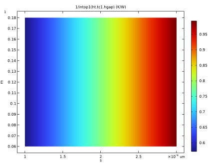
In the Settings window for Global Evaluation, type Constriction Resistance (s, m) in the Label text field.
3
Locate the Data section. From the Dataset list, choose Study 2/Solution 2 (sol2).
4
Locate the Expressions section. In the table, enter the following settings:
5
Click  Evaluate.
Table 1
1
Go to the Table 1 window.
Reproduce Figure 5 as follows.
2
Click the Table Surface button in the window toolbar.
Results
Constriction Resistance (s, m)
1
In the Model Builder window, under Results click 2D Plot Group 2.
2
In the Settings window for 2D Plot Group, type Constriction Resistance (s, m) in the Label text field.
3
Click the  Zoom Extents button in the Graphics toolbar.
Gap Resistance (s, m)
1
In the Results toolbar, click  Global Evaluation.
2
In the Settings window for Global Evaluation, type Gap Resistance (s, m) in the Label text field.
3
Locate the Data section. From the Dataset list, choose Study 2/Solution 2 (sol2).
4
Locate the Expressions section. In the table, enter the following settings:
5
Click  Evaluate.
Table 2
1
Go to the Table 2 window.
2
Click the Table Surface button in the window toolbar.
Results
Gap Resistance (s, m)
1
In the Model Builder window, under Results click 2D Plot Group 3.
2
In the Settings window for 2D Plot Group, type Gap Resistance (s, m) in the Label text field.
3
Click the  Zoom Extents button in the Graphics toolbar.
Add Study
1
In the Home toolbar, click  Add Study to open the Add Study window.
2
Go to the Add Study window.
3
Find the Studies subsection. In the Select Study tree, select General Studies > Stationary.
4
Click the Add Study button in the window toolbar.
5
In the Home toolbar, click  Add Study to close the Add Study window.
Study 3
Parametric Sweep
1
In the Study toolbar, click  Parametric Sweep.
2
In the Settings window for Parametric Sweep, locate the Study Settings section.
3
From the Sweep type list, choose All combinations.
4
5
From the list in the Parameter name column, choose p (Contact pressure), then specify values and unit as follows:
6
7
From the list in the Parameter name column, choose Hmic (Aluminum microhardness), then specify values and unit as follows:
For assistance in entering ranges of different kinds in the Parameter value list column, click the Range button to launch the Range dialog.
8
In the Model Builder window, click Study 3.
9
In the Settings window for Study, locate the Study Settings section.
10
Clear the Generate default plots checkbox.
11
In the Study toolbar, click  Compute.
Results
Constriction Resistance (p, Hmic)
1
In the Results toolbar, click  Global Evaluation.
2
In the Settings window for Global Evaluation, type Constriction Resistance (p, Hmic) in the Label text field.
3
Locate the Data section. From the Dataset list, choose Study 3/Solution 3 (sol3).
4
Locate the Expressions section. In the table, enter the following settings:
5
Click  Evaluate.
Table 3
1
Go to the Table 3 window.
2
Click the Table Surface button in the window toolbar.
Results
Constriction Resistance (p, Hmic)
1
In the Model Builder window, under Results click 2D Plot Group 4.
2
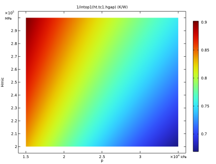
In the Settings window for 2D Plot Group, type Constriction Resistance (p, Hmic) in the Label text field.
3
Click the  Zoom Extents button in the Graphics toolbar.
Gap Resistance (p, Hmic)
1
In the Results toolbar, click  Global Evaluation.
2
In the Settings window for Global Evaluation, type Gap Resistance (p, Hmic) in the Label text field.
3
Locate the Data section. From the Dataset list, choose Study 3/Solution 3 (sol3).
4
Locate the Expressions section. In the table, enter the following settings:
5
Click  Evaluate.
Table 4
1
Go to the Table 4 window.
2
Click the Table Surface button in the window toolbar.
Results
Gap Resistance (p, Hmic)
1
In the Model Builder window, under Results click 2D Plot Group 5.
2
In the Settings window for 2D Plot Group, type Gap Resistance (p, Hmic) in the Label text field.
3
Click the  Zoom Extents button in the Graphics toolbar.
In order to visualize the temperature on each side of the thermal contact, follow the next steps.
Result Templates
1
In the Results toolbar, click  Result Templates to open the Result Templates window.
2
Go to the Result Templates window.
3
In the tree, select Study 1/Solution 1 (sol1) > Heat Transfer in Solids > Contact Temperature (ht).
4
Click the Add Result Template button in the window toolbar.
5
In the Results toolbar, click  Result Templates to close the Result Templates window.
Results
Contact Temperature (ht)
1
In the Settings window for 3D Plot Group, locate the Data section.
2
From the Dataset list, choose Sector 3D 1.