PDF

Convection Cooking of Chicken Patties
Introduction
This example models the convection cooking of a chicken patty. The model was originally developed by H. Chen and others (Ref. 1).
To increase consumer convenience, many of today’s food products are precooked so that you can quickly re-heat the product, for example in a microwave oven. One industrial precooking method is air-convection cooking. This example builds a time-dependent model of the convection cooking process for a chicken patty, and it shows the temperature rise over time in the patty.
This simulation also models the moisture concentration in the patty. From the viewpoint of product quality, it is of interest to minimize the loss of moisture during cooking. In this regard, cooking yield is a quantity that measures how much moisture, in percent, remains in the patty after the cooking process. Furthermore, the moisture concentration also influences the temperature field by heat loss due to vaporization and also by changing the patty’s thermal conductivity.
Figure 1: Convection cooking of a chicken patty.
Model Definition
This COMSOL Multiphysics example couples time-dependent interfaces describing the temperature and the moisture concentration, respectively. The simulation does not model the convective velocity field outside the patty because the coefficients for convective heat and moisture transfer to the surrounding air are given.
Inside the patty, diffusive processes describe both heat transfer and moisture transport.
The model assumes that the specific heat capacity increases with temperature according to the expression
where ΔT = (T − 0°C) and the dimensions of the numerical coefficients are such that the dimension of Cp is as stated.
Figure 2 depicts the patty’s geometry, which is simple and allows for 2D axisymmetric modeling of its cross section. Additional symmetry in the cross section makes it possible to model just one quarter of the cross section.
Figure 2: Geometry of the chicken patty.
These simplifications result in a simple rectangular domain with the dimension 31 mm-by-5 mm. Figure 3 describes the boundary numbering used when specifying the boundary conditions.
Figure 3: Model domain and boundary numbering.
The equations describing moisture diffusion are coupled to the heat equation in the following two ways:
The thermal conductivity, k, increases with moisture concentration according to k = (0.194 + 0.436 (cMH2O ⁄ ρ)) W/(m·K), where c is the concentration (mol/m3), MH2O the molar mass of water (kg/mol) and ρ is the density (kg/m3).
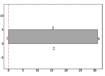
The vaporization of water at the patty’s outer boundaries generates a heat flux out of the patty. Represent this heat flux with the term λDc in the boundary conditions for Boundaries 3 and 4, where λ is the molar latent heat of vaporization (J/mol).
Assume symmetry for the temperature field on Boundaries 1 and 2. Air convection adds heat on Boundaries 3 and 4. According to the assumptions made earlier, add a term for the heat flux out of the patty due to moisture vaporization on Boundaries 3 and 4.
Summarizing, the boundary conditions for the heat transfer interface are
where hT is the heat transfer coefficient (W/(m2·K)), and Tair is the oven air temperature.
The boundary conditions for the diffusion are
where D is the moisture diffusion coefficient in the patty (m2/s), kc refers to the mass transfer coefficient (m/s), and cb denotes the outside air (bulk) moisture concentration (mol/m3). The diffusion coefficient and the mass transfer coefficient are given, respectively, by
where Cm equals the specific moisture capacity (kg moisture/kg meat), km refers to the moisture conductivity (kg/(m·s)), and hm denotes the mass transfer coefficient in mass units (kg/(m2·s)).
Assume that the patty’s temperature is 22°C at the start of the cooking process, and the moisture concentration in the patty at the air interface is 1222 mol/m3 = 22 kg/m3 on a wet basis, which means that the moisture is expressed in mass per volume of meat. Additional data are given in the modeling section below.
To obtain the temperature and moisture concentration over time, the model solves the equations with the boundary conditions discussed above.
Results and Discussion
The most interesting result from this simulation is the time required to heat the patty from room temperature (22°C) to at least 70°C throughout the entire patty. The section at the middle of the patty (at the lower-left corner of the modeling domain) takes the longest time to reach this temperature. It is also interesting to determine how much moisture remains in the patty after cooking. For this purpose, compute the cooking yield, defined as (initial moisture mass)/(final moisture mass).
The model shows that at an oven air temperature of 135°C, a cooking time of approximately 770 s is required to reach a center temperature of 70°C. Figure 4 shows how the temperature increases over time.
Figure 4: Temperature increase over time in the middle of the patty at an air temperature of 135°C.
Figure 5 illustrates the resulting temperature field after 770 s. The temperature at the lower-left corner is 70°C, and the temperature rises toward the outside boundaries.
Figure 5: Temperature field after 770 s at a cooking temperature of 135°C.
At this oven air temperature, the cooking yield is approximately 0.94 (94%). Figure 6 shows the resulting moisture concentration for these conditions. As expected, the convective loss of moisture at the boundaries results in a lower moisture concentration at the outer parts of the patty compared to its inner parts.
Figure 6: Moisture concentration after 770 s at a cooking temperature of 135°C.
Simulations show that an increased air temperature both shortens the time required to reach 70°C in the middle and increases the cooking yield. The drawback, however, is that the temperature gradients in the chicken patty increase. Figure 7 shows the temperature field obtained after 370 s at a cooking temperature of 219°C; the corresponding cooking yield is approximately 0.97 (97%).
Figure 7: Temperature field after 370 s at a cooking temperature of 219°C.
Reference
1. H. Chen, B.P. Marks, and R.Y. Murphy, “Modeling Coupled Heat and Mass Transfer for Convection Cooking of Chicken Patties,” J. Food Engineering, vol. 42, pp. 139–146, 1999.
Application Library path: Heat_Transfer_Module/Phase_Change/chicken_patties
Modeling Instructions
From the File menu, choose New.
New
In the New window, click  Model Wizard.
Model Wizard
1
In the Model Wizard window, click  2D Axisymmetric.
2
In the Select Physics tree, select Chemical Species Transport > Transport of Diluted Species (tds).
3
Click Add.
4
In the Select Physics tree, select Heat Transfer > Heat Transfer in Solids (ht).
5
Click Add.
6
Click  Study.
7
In the Select Study tree, select General Studies > Time Dependent.
8
Global Definitions
Parameters 1
1
In the Model Builder window, under Global Definitions click Parameters 1.
2
In the Settings window for Parameters, locate the Parameters section.
3
Geometry 1
1
In the Model Builder window, under Component 1 (comp1) click Geometry 1.
2
In the Settings window for Geometry, locate the Units section.
3
From the Length unit list, choose mm.
Rectangle 1 (r1)
1
In the Geometry toolbar, click  Rectangle.
2
In the Settings window for Rectangle, locate the Size and Shape section.
3
In the Width text field, type 31.
4
In the Height text field, type 5.
5
In the Geometry toolbar, click  Build All.
6
Click the  Zoom Extents button in the Graphics toolbar.
Definitions
Variables 1
1
In the Definitions toolbar, click  Local Variables.
2
In the Settings window for Variables, locate the Variables section.
3
Materials
Chicken Meat
1
In the Materials toolbar, click  Blank Material.
2
In the Settings window for Material, type Chicken Meat in the Label text field.
3
Locate the Material Contents section. In the table, enter the following settings:
Transport of Diluted Species (tds)
1
In the Model Builder window, under Component 1 (comp1) click Transport of Diluted Species (tds).
2
In the Settings window for Transport of Diluted Species, locate the Transport Mechanisms section.
3
Clear the Convection checkbox.
Fluid 1
1
In the Model Builder window, under Component 1 (comp1) > Transport of Diluted Species (tds) click Fluid 1.
2
In the Settings window for Fluid, locate the Diffusion section.
3
In the Dc text field, type D.
Initial Values 1
1
In the Model Builder window, click Initial Values 1.
2
In the Settings window for Initial Values, locate the Initial Values section.
3
In the c text field, type c0.
Flux 1
1
In the Physics toolbar, click  Boundaries and choose Flux.
2
3
In the Settings window for Flux, locate the Inward Flux section.
4
Select the Species c checkbox.
5
From the Flux type list, choose External convection.
6
In the kc,c text field, type k_c.
7
In the cb,c text field, type c_b.
Heat Transfer in Solids (ht)
Initial Values 1
1
In the Model Builder window, under Component 1 (comp1) > Heat Transfer in Solids (ht) click Initial Values 1.
2
In the Settings window for Initial Values, locate the Initial Values section.
3
In the T text field, type T0.
Heat Flux 1
1
In the Physics toolbar, click  Boundaries and choose Heat Flux.
2
3
In the Settings window for Heat Flux, locate the Heat Flux section.
4
From the Flux type list, choose Convective heat flux.
5
In the h text field, type h_T.
6
In the Text text field, type T_air.
Boundary Heat Source 1
1
In the Physics toolbar, click  Boundaries and choose Boundary Heat Source.
2
3
In the Settings window for Boundary Heat Source, locate the Boundary Heat Source section.
4
In the Qb text field, type lda*k_c*(c_b-c).
Mesh 1
Free Triangular 1
In the Mesh toolbar, click  Free Triangular.
Size 1
1
Right-click Free Triangular 1 and choose Size.
2
In the Settings window for Size, locate the Geometric Entity Selection section.
3
From the Geometric entity level list, choose Boundary.
4
5
Locate the Element Size section. Click the Custom button.
6
Locate the Element Size Parameters section.
7
Select the Maximum element size checkbox. In the associated text field, type 0.1.
8
Click  Build All.
Study 1
Step 1: Time Dependent
1
In the Model Builder window, under Study 1 click Step 1: Time Dependent.
2
In the Settings window for Time Dependent, locate the Study Settings section.
3
In the Output times text field, type range(0,10,900).
4
In the Study toolbar, click  Compute.
Change the unit of the temperature results to degrees Celsius.
Results
Preferred Units 1
1
In the Results toolbar, click  Configurations and choose Preferred Units.
2
In the Settings window for Preferred Units, locate the Units section.
3
Click  Add Physical Quantity.
4
In the Physical Quantity dialog, select General > Temperature (K) in the tree.
5
6
In the Settings window for Preferred Units, locate the Units section.
7
8
Click  Apply.
The first two default plots visualize the moisture content at the last time step in 2D and 3D. The third default plot shows the temperature in 2D. To plot the change of the temperature in time in the middle of the patty (Figure 4), follow the steps given below.
Temperature Profile vs. Time
1
In the Results toolbar, click  1D Plot Group.
2
In the Settings window for 1D Plot Group, type Temperature Profile vs. Time in the Label text field.
Point Graph 1
1
In the Temperature Profile vs. Time toolbar, click  Point Graph.
2
3
In the Settings window for Point Graph, click Replace Expression in the upper-right corner of the y-Axis Data section. From the menu, choose Component 1 (comp1) > Heat Transfer in Solids > Temperature > T - Temperature - K.
4
In the Temperature Profile vs. Time toolbar, click  Plot.
It takes 770 s to reach a temperature of 70°C in the center. Plot the temperature and moisture distributions in the patty for the time value 770 s (Figure 5 and Figure 6).
Concentration (tds)
1
In the Model Builder window, click Concentration (tds).
2
In the Settings window for 2D Plot Group, locate the Data section.
3
From the Time (s) list, choose 770.
4
In the Concentration (tds) toolbar, click  Plot.
Temperature (ht)
1
In the Model Builder window, click Temperature (ht).
2
In the Settings window for 2D Plot Group, locate the Data section.
3
From the Time (s) list, choose 770.
4
In the Temperature (ht) toolbar, click  Plot.
Now, compute the cooking yield.
Volume Average 1
1
In the Results toolbar, click  More Derived Values and choose Average > Volume Average.
2
In the Settings window for Volume Average, locate the Data section.
3
From the Time selection list, choose From list.
4
In the Times (s) list box, select 770.
5
Locate the Expressions section. In the table, enter the following settings:
6
Click  Evaluate.
Study 1
To study the evolution of the temperature and the moisture in the patty for a range of oven temperatures, use the parametric solver.
Parametric Sweep
1
In the Study toolbar, click  Parametric Sweep.
2
In the Settings window for Parametric Sweep, locate the Study Settings section.
3
4
5
In the Study toolbar, click  Compute.
Results
Examine the temperature rise in the middle of the patty for the different oven temperature values.
Temperature Profile vs. Time
1
In the Model Builder window, under Results click Temperature Profile vs. Time.
2
In the Settings window for 1D Plot Group, locate the Data section.
3
From the Dataset list, choose Study 1/Parametric Solutions 1 (sol2).
4
Locate the Legend section. From the Position list, choose Lower right.
Point Graph 1
1
In the Model Builder window, click Point Graph 1.
2
In the Settings window for Point Graph, locate the x-Axis Data section.
3
From the Axis source data list, choose Inner solutions.
4
Click to expand the Legends section. Select the Show legends checkbox.
5
From the Legends list, choose Evaluated.
6
In the Legend text field, type Air temperature at eval(T_air,degC)°C.
7
In the Temperature Profile vs. Time toolbar, click  Plot.
Follow these steps to see the temperature distribution inside the patty for the oven temperature 219°C. Compare the resulting plot with that in Figure 7.
Temperature (ht) 1
1
In the Model Builder window, under Results click Temperature (ht) 1.
2
In the Settings window for 2D Plot Group, locate the Data section.
3
From the Time (s) list, choose 370.
4
In the Temperature (ht) 1 toolbar, click  Plot.
Finally, compute the cooking yield.
Volume Average 2
1
In the Results toolbar, click  More Derived Values and choose Average > Volume Average.
2
In the Settings window for Volume Average, locate the Data section.
3
From the Dataset list, choose Revolution 2D 2.
4
From the Parameter selection (T_air) list, choose From list.
5
In the Parameter values (T_air (degC)) list box, select 219.
6
From the Time selection list, choose From list.
7
In the Times (s) list box, select 370.
8
From the Table columns list, choose T_air.
9
Locate the Expressions section. In the table, enter the following settings:
10
Click  Evaluate.