PDF

Failure of a Concrete Beam Using Coupled Damage–Plasticity
Introduction
Failure of reinforced concrete structures involves advanced material behavior and interaction between materials. This example demonstrates how to model various stages of the failure of a reinforced concrete beam by including a coupled damage–plasticity material model for the concrete, metal plasticity for the rebars, and a nonlinear bond-slip law for the interaction between concrete and the rebar.
Model Definition
The example aims to model a simply supported reinforced concrete beam subjected to two distributed loads. The total length of the beam is 4.5 m, and the cross section is 200 mm wide and 300 mm high. A geometrical reinforcement content equal to 4.5% is used, with the rebar placed 50 mm from the bottom of the beam
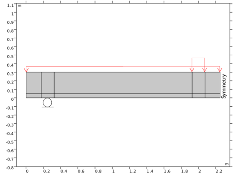
The geometry is defined in 2D with an assumption of plane stress, and a symmetry plane is utilized so that only half of the beam is modeled. Figure 1 shows the geometry and a schematic description of the boundary conditions. Since a 2D geometry is used, the entire reinforcement content is assumed to be lumped in a single edge, where truss elements are inserted with the appropriate cross-section area.
Figure 1: Model geometry and boundary conditions.
Properties of the concrete material are given in Table 1. All other parameters necessary to define the coupled damage–plasticity model are set to their default. The reinforcement is defined as an elastoplastic material with linear isotropic hardening. Table 2 lists its material properties.
ν
σuc
σut
Gft
ν
σys
ETiso
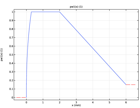
To accurately describe the failure process of reinforced concrete structures, it is important to also consider the interaction between concrete and rebar, often referred to as a bond-slip law. The interaction can be severely nonlinear and have a large impact on how cracks form and on the overall failure mechanism. In this example, the interaction is modeled by inserting distributed springs between the truss mesh elements of the rebar and the solid mesh elements of the concrete. In order to include the bond-slip law, a friction model is added to the otherwise elastic springs in the axial direction of the rebar. Any bond-slip law can here be included by adding a user-defined hardening model to the cohesion that determines when slip occurs. Here a hardening model according to Figure 2 is implemented, which is similar to what can be found in many model and design codes for concrete structures.
Figure 2: Hardening model used for the bond-slip law. Note that the y-axis is a normalized measure of the bond strength.
The analysis is set up as a parametric sweep such that the load is incrementally increased to capture the entire failure process.
Results and Discussion
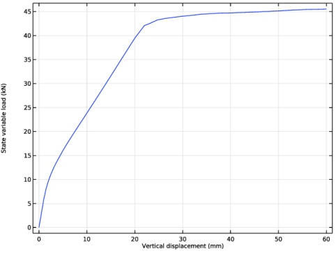
The total load applied to the beam is monitored by a Probe that stores its value at every step taken by the solver to show extra detail. Figure 3 shows the resulting curve. Here one can clearly distinguish three different stages:
Figure 3: Load versus displacement curve of the reinforced concrete beam.
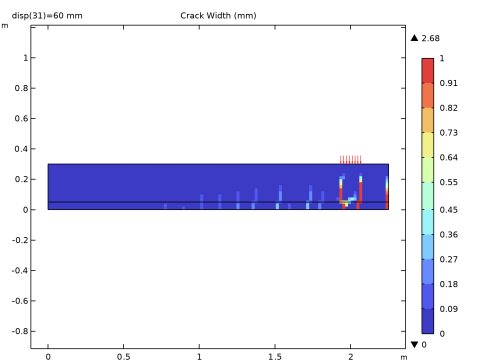
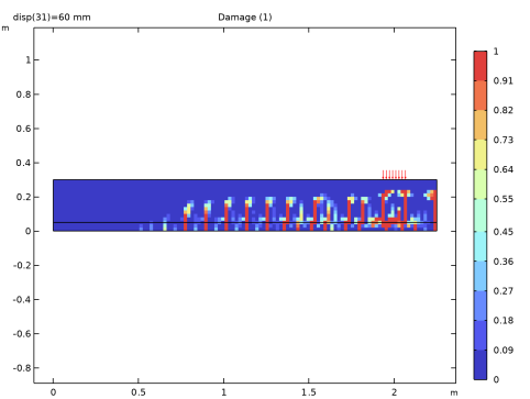
The cracks previously mentioned can be seen in Figure 4, which shows an estimate of the crack width at the last step of the analysis. Here one can clearly see that most of the deformation is localized to the cracks near the midsection, where the crack width exceeds 1 mm. Observe, however, that the stiffness is lost in all cracks as indicated by Figure 5, which shows the damage.
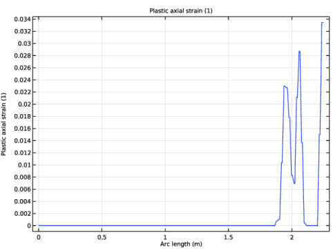
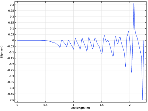
The reason why most deformation is localized in some of the cracks is due to yielding of the reinforcement. As shown in Figure 6, the plastic deformation is concentrated bands close to the midsection. Here, an effect of the bond-slip model is seen since the plastic bands clearly extend to more than the single mesh element of the crack. The computed slip is shown in Figure 7.
Figure 4: Estimated crack width at the last step of the analysis.
Figure 5: Damage at the last step of the analysis.
Figure 6: Plastic deformation in the reinforcement at the last step of the analysis.
Figure 7: Slip between concrete and the rebar at the last step of the analysis.
Notes About the COMSOL Implementation
Failure of concrete and reinforced concrete structures is a very nonlinear process, and we cannot expect any boundary loads to be monotonically increasing. Hence, any distributed load needs to be indirectly controlled by some other measure. Here, the vertical displacement at the midsection of the beam is used as a control variable in a Global equation. This algebraic equation is used to compute a load proportionality factor.
When the crack-band method is used as a spatial regularization method to model softening, symmetry conditions need special attention. In principle, the crack-band width is doubled for mesh elements next to a symmetry plane. In order not to overestimate the dissipated energy during softening, it is necessary to compensate for this fact. Here, this is done by reducing the fracture energy Gft by a factor 0.5 for the relevant mesh elements.
The coupled damage–plasticity model requires local computations at each Gauss point during the assembly process, which is expensive. By using Reduced Integration, the number of Gauss points are reduced by a factor four for the given displacement shape-function order and mesh-element type. This setting speeds up the computation time significantly.
Application Library path: Geomechanics_Module/Concrete/concrete_beam_cdpm
Modeling Instructions
From the File menu, choose New.
New
In the New window, click  Model Wizard.
Model Wizard
1
In the Model Wizard window, click  2D.
2
In the Select Physics tree, select Structural Mechanics > Solid Mechanics (solid).
3
Click Add.
4
In the Select Physics tree, select Structural Mechanics > Truss (truss).
5
Click Add.
6
In the Displacement field (m) text field, type u.
7
Click  Study.
8
In the Select Study tree, select General Studies > Stationary.
9
Global Definitions
Parameters 1
1
In the Model Builder window, under Global Definitions click Parameters 1.
2
In the Settings window for Parameters, locate the Parameters section.
3
Geometry Parameters
1
In the Home toolbar, click  Parameters and choose Add > Parameters.
2
In the Settings window for Parameters, type Geometry Parameters in the Label text field.
3
Locate the Parameters section. In the table, enter the following settings:
Geometry 1
Rectangle 1 (r1)
1
In the Geometry toolbar, click  Rectangle.
2
In the Settings window for Rectangle, locate the Size and Shape section.
3
In the Width text field, type length.
4
In the Height text field, type height.
5
Click to expand the Layers section. In the table, enter the following settings:
6
Clear the Layers on bottom checkbox.
7
Select the Layers to the left checkbox.
Polygon 1 (pol1)
1
In the Geometry toolbar, click  Polygon.
2
In the Settings window for Polygon, locate the Coordinates section.
3
Form Union (fin)
1
In the Model Builder window, under Component 1 (comp1) > Geometry 1 click Form Union (fin).
2
In the Settings window for Form Union/Assembly, locate the Form Union/Assembly section.
3
From the Action list, choose Form an assembly.
Mesh Control Edges 1 (mce1)
1
In the Geometry toolbar, click  Virtual Operations and choose Mesh Control Edges.
2
On the object fin, select Boundaries 4, 7, 10, and 13 only.
3
In the Settings window for Mesh Control Edges, locate the Input section.
4
Clear the Include adjacent vertices checkbox.
Mesh Control Vertices 1 (mcv1)
1
In the Geometry toolbar, click  Virtual Operations and choose Mesh Control Vertices.
2
On the object mce1, select Points 4, 6, 7, and 9 only.
3
In the Geometry toolbar, click  Build All.
Solid Mechanics (solid)
1
In the Model Builder window, under Component 1 (comp1) click Solid Mechanics (solid).
2
In the Settings window for Solid Mechanics, locate the 2D Approximation section.
3
4
Locate the Thickness section. In the d text field, type width.
It is recommended to use a linear displacement field when the model includes a material model based on damage.
5
Click to expand the Discretization section. From the Displacement field list, choose Linear.
Linear Elastic Material 1
The local computations at Gauss points during assembly are expensive for the coupled damage-plasticity concrete model. Using a reduced integration scheme will reduce the overall simulation time.
1
In the Model Builder window, under Component 1 (comp1) > Solid Mechanics (solid) click Linear Elastic Material 1.
2
In the Settings window for Linear Elastic Material, locate the Quadrature Settings section.
3
Select the Reduced integration checkbox.
Concrete 1
1
In the Physics toolbar, click  Attributes and choose Concrete.
2
In the Settings window for Concrete, locate the Concrete Model section.
3
From the Material model list, choose Coupled damage–plasticity.
4
Find the Tension softening subsection. From the list, choose Cornelissen.
5
Find the Compression softening subsection. In the εfc text field, type 5e-3.
Symmetry 1
1
In the Physics toolbar, click  Boundaries and choose Symmetry.
2
Rigid Connector 1
1
In the Physics toolbar, click  Boundaries and choose Rigid Connector.
2
3
In the Settings window for Rigid Connector, locate the Prescribed Displacement at Center of Rotation section.
4
Select the Prescribed in y direction checkbox.
The distributed loads will be added by indirect displacement control, forcing the displacement of a control point to be monotonically increasing.
Definitions
Integration 1 (intop1)
1
In the Definitions toolbar, click  Nonlocal Couplings and choose Integration.
2
In the Settings window for Integration, locate the Source Selection section.
3
From the Geometric entity level list, choose Point.
4
5
Click the  Show More Options button in the Model Builder toolbar.
6
In the Show More Options dialog, in the tree, select the checkbox for the node Physics > Equation Contributions.
7
Solid Mechanics (solid)
Global Equations 1 (ODE1)
1
In the Physics toolbar, click  Global and choose Global Equations.
2
In the Settings window for Global Equations, locate the Global Equations section.
3
4
Locate the Units section. Click  Select Dependent Variable Quantity.
5
In the Physical Quantity dialog, type force in the text field.
6
In the tree, select General > Force (N).
7
8
In the Settings window for Global Equations, locate the Units section.
9
Click  Select Source Term Quantity.
10
In the Physical Quantity dialog, type disp in the text field.
11
In the tree, select General > Displacement (m).
12
Boundary Load 1
1
In the Physics toolbar, click  Boundaries and choose Boundary Load.
2
3
In the Settings window for Boundary Load, locate the Force section.
4
From the Load type list, choose Total force.
5
Specify the Ftot vector as
Boundary Load 2
1
In the Physics toolbar, click  Boundaries and choose Boundary Load.
2
3
In the Settings window for Boundary Load, locate the Force section.
4
From the Load type list, choose Total force.
5
Specify the Ftot vector as
Truss (truss)
1
In the Model Builder window, under Component 1 (comp1) click Truss (truss).
2
Linear Elastic Material 1
In the Model Builder window, under Component 1 (comp1) > Truss (truss) click Linear Elastic Material 1.
Plasticity 1
In the Physics toolbar, click  Attributes and choose Plasticity.
Cross-Section Data 1
The reinforced beam is assumed to have a geometrical reinforcement content equal to 0.8%.
1
In the Model Builder window, under Component 1 (comp1) > Truss (truss) click Cross-Section Data 1.
2
In the Settings window for Cross-Section Data, locate the Cross-Section Definition section.
3
In the A text field, type height*width*0.8[%].
Symmetry 1
1
In the Physics toolbar, click  Points and choose Symmetry.
2
Multiphysics
Embedded Reinforcement 1 (ere1)
1
In the Physics toolbar, click  Multiphysics Couplings and choose Global > Embedded Reinforcement.
2
In the Settings window for Embedded Reinforcement, locate the Edge Selection, Embedded Structure section.
3
Click to select the  Activate Selection toggle button.
4
The default spring stiffness leads to an ill-condition system of equations. Use a lower value to avoid this.
5
Locate the Connection Settings section. From the Connection type list, choose Spring constant per reference area.
6
In the ka text field, type ((1e-1*ere1.Eequ)*ere1.perimeter)/(h^2).
7
In the kt text field, type ((1e1*ere1.Eequ)*ere1.perimeter)/(h^2).
Add a bond-slip law. A typical bond-slip curve for concrete is most easily implemented as a user-defined hardening model using a Piecewise function.
8
Find the Bond slip model subsection. From the list, choose Friction.
9
In the c0 text field, type 1[MPa].
Definitions
Piecewise 1 (pw1)
1
In the Definitions toolbar, click  Piecewise.
2
In the Settings window for Piecewise, locate the Units section.
3
In the Arguments text field, type mm.
4
In the Function text field, type 1.
5
Locate the Definition section. Find the Intervals subsection. In the table, enter the following settings:
6
Multiphysics
Embedded Reinforcement 1 (ere1)
1
In the Model Builder window, under Component 1 (comp1) > Multiphysics click Embedded Reinforcement 1 (ere1).
2
In the Settings window for Embedded Reinforcement, locate the Connection Settings section.
3
Find the Bond slip model subsection. From the Hardening model list, choose User defined.
4
In the c  h text field, type 5[MPa]*pw1(ere1.upe).
Materials
Material 1 (mat1)
1
In the Model Builder window, under Component 1 (comp1) right-click Materials and choose Blank Material.
2
In the Settings window for Material, locate the Material Contents section.
3
The crack-band width is doubled for mesh elements next to a symmetry plane. Reduce the fracture energy in such mesh elements to compensate.
Definitions
Analytic 1 (an1)
1
In the Definitions toolbar, click  Analytic.
2
In the Settings window for Analytic, locate the Definition section.
3
In the Expression text field, type if(x>=length-1.05*meshSize/2,1/2,1).
4
Locate the Units section. In the Function text field, type 1.
5
Materials
Material 1 (mat1)
1
In the Model Builder window, under Component 1 (comp1) > Materials click Material 1 (mat1).
2
In the Settings window for Material, locate the Material Contents section.
3
Material 2 (mat2)
1
In the Model Builder window, right-click Materials and choose Blank Material.
2
In the Settings window for Material, locate the Geometric Entity Selection section.
3
From the Geometric entity level list, choose Boundary.
4
5
Locate the Material Contents section. In the table, enter the following settings:
Mesh 1
Mapped 1
In the Mesh toolbar, click  Mapped.
Edge 1
1
In the Mesh toolbar, click  More Generators and choose Edge.
2
Size
1
In the Model Builder window, click Size.
2
In the Settings window for Size, locate the Element Size section.
3
Click the Custom button.
4
Locate the Element Size Parameters section. In the Maximum element size text field, type meshSize.
5
Click  Build All.
Study 1
Step 1: Stationary
1
In the Model Builder window, under Study 1 click Step 1: Stationary.
2
In the Settings window for Stationary, click to expand the Study Extensions section.
3
Select the Auxiliary sweep checkbox.
4
5
Show the default solver in order to make some modifications to the automatic suggestion.
Solution 1 (sol1)
1
In the Study toolbar, click  Show Default Solver.
2
In the Model Builder window, expand the Solution 1 (sol1) node.
3
In the Model Builder window, expand the Study 1 > Solver Configurations > Solution 1 (sol1) > Stationary Solver 1 node, then click Parametric 1.
4
In the Settings window for Parametric, click to expand the Continuation section.
5
Select the Tuning of step size checkbox.
6
In the Initial step size text field, type 1e-3.
7
In the Minimum step size text field, type 1e-8.
8
In the Maximum step size text field, type 2e-3.
9
Locate the General section. From the On error list, choose Skip parameter step.
10
In the Model Builder window, under Study 1 > Solver Configurations > Solution 1 (sol1) > Stationary Solver 1 click Fully Coupled 1.
11
In the Settings window for Fully Coupled, click to expand the Method and Termination section.
12
In the Tolerance factor text field, type 1.0e-1.
Add a Global Variable Probe to monitor the solution while solving.
Definitions
Global Variable Probe 1 (var1)
1
In the Definitions toolbar, click  Probes and choose Global Variable Probe.
2
In the Settings window for Global Variable Probe, locate the Expression section.
3
In the Expression text field, type load.
4
From the Table and plot unit list, choose kN.
Also, show the default plots and add a Damage plot from Result Templates to monitor the solution while solving.
Study 1
In the Study toolbar, click  Show Default Plots.
Result Templates
1
In the Results toolbar, click  Result Templates to open the Result Templates window.
2
Go to the Result Templates window.
3
In the tree, select Study 1/Solution 1 (sol1) > Solid Mechanics (solid) > Damage (solid).
4
Click the Add Result Template button in the window toolbar.
5
In the Results toolbar, click  Result Templates to close the Result Templates window.
Study 1
Step 1: Stationary
1
In the Settings window for Stationary, click to expand the Results While Solving section.
2
Select the Plot checkbox.
3
4
From the Update at list, choose Steps taken by solver.
5
In the Study toolbar, click  Compute.
Results
Probe Plot Group 1
1
In the Model Builder window, under Results click Probe Plot Group 1.
2
In the Settings window for 1D Plot Group, locate the Plot Settings section.
3
Select the x-axis label checkbox. In the associated text field, type Vertical displacement (mm).
4
Locate the Legend section. Clear the Show legends checkbox.
5
In the Probe Plot Group 1 toolbar, click  Plot.
The default stress plot shows the undamaged von Mises stress, it is of greater interest to show a component of the damaged stress tensor.
Surface 1
1
In the Model Builder window, expand the Results > Stress (solid) node, then click Surface 1.
2
In the Settings window for Surface, click Replace Expression in the upper-right corner of the Expression section. From the menu, choose Component 1 (comp1) > Solid Mechanics > Damage > Stress tensor, damaged (spatial frame) - N/m² > solid.sdGpxx - Stress tensor, damaged, xx-component.
3
Locate the Expression section. From the Unit list, choose MPa.
4
Locate the Coloring and Style section. From the Color table list, choose Rainbow.
Arrow Line 1
1
In the Model Builder window, right-click Damage (solid) and choose Arrow Line.
2
In the Settings window for Arrow Line, click Replace Expression in the upper-right corner of the Expression section. From the menu, choose Component 1 (comp1) > Solid Mechanics > Load > solid.fax,solid.fay - Force per deformed area (spatial frame).
3
Click to expand the Title section. From the Title type list, choose None.
4
Locate the Arrow Positioning section. From the Placement list, choose Gauss points.
5
Locate the Coloring and Style section. From the Arrow base list, choose Head.
6
In the Damage (solid) toolbar, click  Plot.
Create a plot that shows an estimate of the crack width. Note that this variable should be evaluated at Gauss points.
Damage (solid) 1
Right-click Damage (solid) and choose Duplicate.
Set default units for result presentation.
Preferred Units 1
1
In the Results toolbar, click  Configurations and choose Preferred Units.
2
In the Settings window for Preferred Units, locate the Units section.
3
Click  Add Physical Quantity.
4
In the Physical Quantity dialog, select General > Displacement (m) in the tree.
5
6
In the Settings window for Preferred Units, locate the Units section.
7
8
Select the Apply conversions to expressions with the same dimensions checkbox.
9
Click  Apply.
Crack Width (solid)
1
In the Model Builder window, expand the Results > Damage (solid) 1 node, then click Damage (solid) 1.
2
In the Settings window for 2D Plot Group, type Crack Width (solid) in the Label text field.
3
Locate the Color Legend section. Select the Show maximum and minimum values checkbox.
Surface 1
1
In the Model Builder window, click Surface 1.
2
In the Settings window for Surface, locate the Expression section.
3
In the Expression text field, type solid.gpeval(solid.lemm1.cm1.wdmgt).
4
In the Description text field, type Crack Width.
5
Click to expand the Range section. Select the Manual color range checkbox.
6
In the Maximum text field, type 1.
7
In the Crack Width (solid) toolbar, click  Plot.
Create a plot that shows the plastic strain in the reinforcement.
Plastic Strain (truss)
1
In the Home toolbar, click  Add Plot Group and choose 1D Plot Group.
2
In the Settings window for 1D Plot Group, type Plastic Strain (truss) in the Label text field.
3
Locate the Data section. From the Parameter selection (disp) list, choose Last.
Line Graph 1
1
Right-click Plastic Strain (truss) and choose Line Graph.
2
3
In the Settings window for Line Graph, click Replace Expression in the upper-right corner of the y-Axis Data section. From the menu, choose Component 1 (comp1) > Truss > Strain > truss.epnGp - Plastic axial strain - 1.
4
In the Plastic Strain (truss) toolbar, click  Plot.
Create a plot that shows the slip between the reinforcement and the concrete. Note that this variable should be evaluated at Gauss points.
Slip
1
In the Model Builder window, right-click Plastic Strain (truss) and choose Duplicate.
2
In the Settings window for 1D Plot Group, click to expand the Title section.
3
From the Title type list, choose None.
4
In the Label text field, type Slip.
5
Locate the Plot Settings section.
6
Select the y-axis label checkbox. In the associated text field, type Slip (mm).
Line Graph 1
1
In the Model Builder window, expand the Slip node, then click Line Graph 1.
2
In the Settings window for Line Graph, locate the y-Axis Data section.
3
In the Expression text field, type gpeval(2,ere1.un).
4
In the Slip toolbar, click  Plot.