
PDF

Isolator Thickness Effect
Introduction
Magnesium (Mg) alloy being the lightest structural material is an attractive alternative for light weighting purpose in various engineering fields. However, Mg alloys are prone to galvanic corrosion when they are joined with steel structures (See models - Galvanic Corrosion of a Magnesium Alloy in Contact with Steel and Galvanic Corrosion with Electrode Deformation - which are available in the Application Libraries). Aluminum (Al) alloys are commonly used as isolators to mitigate galvanic corrosion between Mg alloy and steel structures.
This model example simulates the effect of isolator thickness on galvanic corrosion and is based on a paper by Deshpande (Ref. 1).
Model Definition
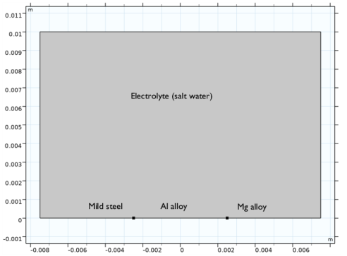
The model geometry considered in this example is shown in Figure 1 where Mg alloy, Al alloy and mild steel (MS), joined together and exposed to the electrolyte, are highlighted. The Al isolator thickness is varied to simulate its effect on galvanic corrosion mitigation.
Use the Secondary Current Distribution interface to solve for the electrolyte potential, ϕl (SI unit: V), over the electrolyte domain according to:
where il (SI unit: A/m2) is the electrolyte current density vector and σl (SI unit: S/m) is the electrolyte conductivity which is assumed to be a constant.
Use the default Insulation condition for all boundaries except the electrode surfaces:
where n is the normal vector, pointing out of the domain.
Figure 1: Model geometry consisting of Mg alloy, Al alloy and mild steel joined together and exposed to the electrolyte solution.
Use the Electrode Surface boundary node at the electrode surfaces which sets the boundary condition for the electrolyte potential according to
where iloc,m (SI unit: A/m2) is the local individual electrode reaction current density.
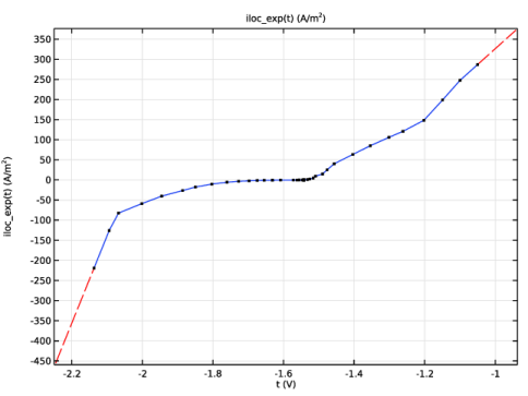
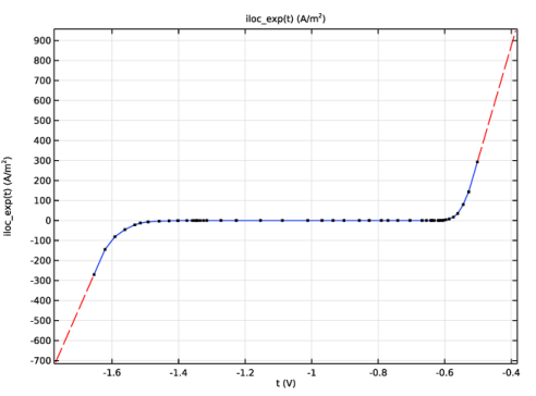
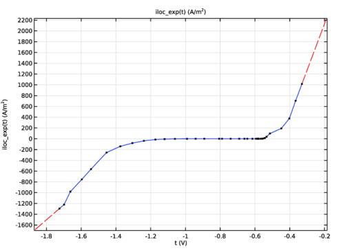
The electrode kinetics at the magnesium alloy, aluminum alloy and mild steel surfaces is described using the experimental polarization data available in corrosion material library, as shown in Figure 2, Figure 3 and Figure 4, respectively.
Figure 2: Polarization data for Mg alloy.
Figure 3: Polarization data for Al alloy.
Figure 4: Polarization data for MS.
Results and Discussion
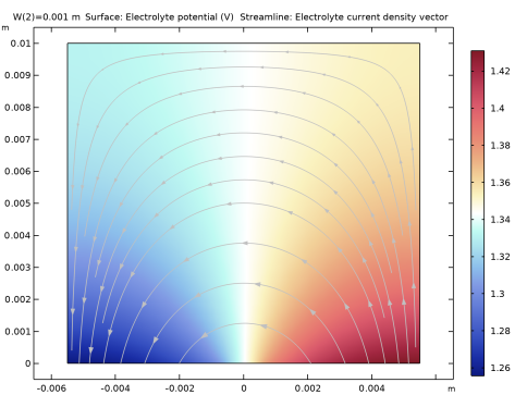
Figure 5 shows a surface plot of the electrolyte potential and a surface arrow plot of the electrolyte current density vector for a magnesium (Mg)–mild steel (MS) galvanic couple with 1 mm thick Al isolator sandwiched between them. The surface arrow plot indicates the electrolyte current density, which in this case coincides with the ionic path taken by the Mg2+ ions that get dissolved in the electrolyte solution from the Mg surface.
Figure 5: A surface plot of the electrolyte potential and surface arrow plot of electrolyte current density vector for 1 mm thick Al isolator.
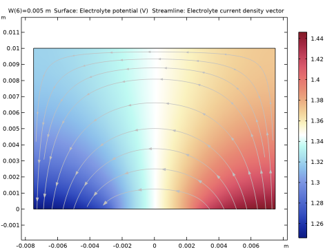
Figure 6 shows a surface plot of the electrolyte potential and a surface arrow plot of the electrolyte current density vector for a magnesium (Mg) - mild steel (MS) galvanic couple with 5 mm thick Al isolator sandwiched between them. The surface arrow plot indicates that the ionic path taken by Mg2+ ions which get dissolved in the electrolyte solution from the Mg electrode surface is longer in case of 5 mm thick Al isolator. The increased distance and hence, IR drop, decreases the galvanic current density at the Mg electrode surface, mitigating galvanic corrosion.
Figure 6: A surface plot of the electrolyte potential and surface arrow plot of electrolyte current density vector for 5 mm thick Al isolator.
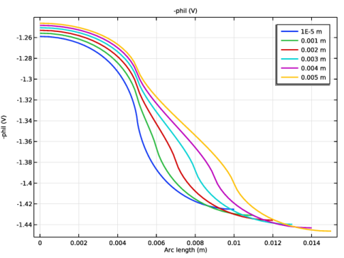
Figure 7 shows the electrolyte potential variation over the electrode surfaces for the varied isolator thicknesses. The Mg surface is the most anodically polarized in case of the thinnest isolator and the least polarized in case of the thickest isolator indicating its corrosion propensity.
Figure 7: Electrolyte potential variation over the electrode surfaces for the varied isolator thicknesses.
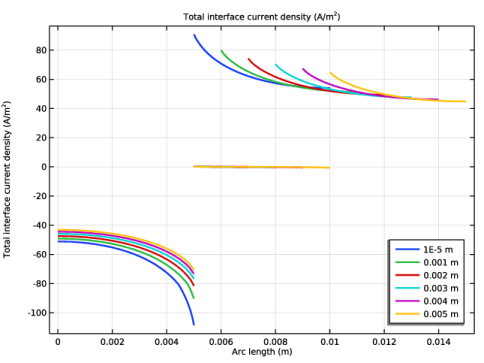
Figure 8 shows the total interface current density variation over the electrode surfaces for the varied isolator thicknesses. The current density over the Mg surface is the highest in case of the thinnest isolator and the lowest in case of the thickest isolator once again indicating its corrosion propensity.
Figure 8: Total interface current density variation over the electrode surfaces for the varied isolator thicknesses.
Notes About the COMSOL Implementation
The Secondary Current Distribution interface is used to model the problem, using Electrode Surface nodes for the three electrode surfaces.
Electrode kinetics is incorporated in the model using the experimental polarization data available in corrosion material library for three electrode surfaces.
A stationary study step is used to solve the problem, with a parametric sweep to vary the isolator thickness.
A free triangular mesh is used for meshing, with a finer resolution at the contact points between different materials.
Reference
1. K.B. Deshpande, “Effect of aluminium spacer on galvanic corrosion between magnesium and mild steel using numerical model and SVET experiments,” Corrosion Science, vol. 62, pp. 184–191, 2012.
Application Library path: Corrosion_Module/Galvanic_Corrosion/isolator_thickness
Modeling Instructions
From the File menu, choose New.
New
In the New window, click  Model Wizard.
Model Wizard
1
In the Model Wizard window, click  2D.
2
In the Select Physics tree, select Electrochemistry > Primary and Secondary Current Distribution > Secondary Current Distribution (cd).
3
Click Add.
4
Click  Study.
5
In the Select Study tree, select General Studies > Stationary.
6
Global Definitions
Add some model parameters.
Parameters 1
1
In the Model Builder window, under Global Definitions click Parameters 1.
2
In the Settings window for Parameters, locate the Parameters section.
3
Geometry 1
Now create the geometry by using a rectangle and two points. The isolator width W is varied using a parametric study.
Rectangle 1 (r1)
1
In the Geometry toolbar, click  Rectangle.
2
In the Settings window for Rectangle, locate the Size and Shape section.
3
In the Width text field, type 0.01+W.
4
In the Height text field, type 0.01.
5
Locate the Position section. In the x text field, type -0.005-W/2.
Point 1 (pt1)
1
In the Geometry toolbar, click  Point.
2
In the Settings window for Point, locate the Point section.
3
In the x text field, type -W/2.
Point 2 (pt2)
1
In the Geometry toolbar, click  Point.
2
In the Settings window for Point, locate the Point section.
3
In the x text field, type W/2.
4
Click  Build All Objects.
5
Click the  Zoom Extents button in the Graphics toolbar.
The geometry should now look like Figure 1 in the documentation.
Materials
Use the Corrosion material library to set up the material properties for the electrode kinetics at the magnesium, aluminum and mild steel electrode surfaces.
Add Material
1
In the Materials toolbar, click  Add Material to open the Add Material window.
2
Go to the Add Material window.
3
In the tree, select Corrosion > Iron Alloys (Steels) > Mild steel in 1.6 wt% NaCl.
4
Click the Add to Component button in the window toolbar.
Materials
Mild steel in 1.6 wt% NaCl (mat1)
1
In the Settings window for Material, locate the Geometric Entity Selection section.
2
From the Geometric entity level list, choose Boundary.
3
4
In the Model Builder window, expand the Mild steel in 1.6 wt% NaCl (mat1) node.
Interpolation 1 (iloc_exp)
1
In the Model Builder window, expand the Component 1 (comp1) > Materials > Mild steel in 1.6 wt% NaCl (mat1) > Local current density (lcd) node, then click Interpolation 1 (iloc_exp).
2
In the Settings window for Interpolation, click  Plot.
Compare the function plot with Figure 4.
Add Material
1
Go to the Add Material window.
2
In the tree, select Corrosion > Aluminum Alloys > AA6063 in 1.6 wt% NaCl.
3
Click the Add to Component button in the window toolbar.
Materials
AA6063 in 1.6 wt% NaCl (mat2)
1
In the Settings window for Material, locate the Geometric Entity Selection section.
2
From the Geometric entity level list, choose Boundary.
3
4
In the Model Builder window, expand the AA6063 in 1.6 wt% NaCl (mat2) node.
Interpolation 1 (iloc_exp)
1
In the Model Builder window, expand the Component 1 (comp1) > Materials > AA6063 in 1.6 wt% NaCl (mat2) > Local current density (lcd) node, then click Interpolation 1 (iloc_exp).
2
In the Settings window for Interpolation, click  Plot.
Compare the function plot with Figure 3.
Add Material
1
Go to the Add Material window.
2
In the tree, select Corrosion > Magnesium Alloys > AE44 in 1.6 wt% NaCl.
3
Click the Add to Component button in the window toolbar.
Materials
AE44 in 1.6 wt% NaCl (mat3)
1
In the Settings window for Material, locate the Geometric Entity Selection section.
2
From the Geometric entity level list, choose Boundary.
3
4
In the Model Builder window, expand the AE44 in 1.6 wt% NaCl (mat3) node.
Interpolation 1 (iloc_exp)
1
In the Model Builder window, expand the Component 1 (comp1) > Materials > AE44 in 1.6 wt% NaCl (mat3) > Local current density (lcd) node, then click Interpolation 1 (iloc_exp).
2
In the Settings window for Interpolation, click  Plot.
Compare the function plot with Figure 2.
3
In the Materials toolbar, click  Add Material to close the Add Material window.
Secondary Current Distribution (cd)
Now set up the physics for the current distribution. Start with selecting the reference electrode potential.
1
In the Settings window for Secondary Current Distribution, click to expand the Physics vs. Materials Reference Electrode Potential section.
2
From the list, choose 0.241 V (SCE vs. SHE).
Electrolyte 1
1
In the Model Builder window, under Component 1 (comp1) > Secondary Current Distribution (cd) click Electrolyte 1.
2
In the Settings window for Electrolyte, locate the Electrolyte section.
3
From the σl list, choose User defined. In the associated text field, type sigma.
Electrode Surface 1
1
In the Physics toolbar, click  Boundaries and choose Electrode Surface.
2
Electrode Reaction 1
1
In the Model Builder window, click Electrode Reaction 1.
2
In the Settings window for Electrode Reaction, locate the Electrode Kinetics section.
3
From the iloc,expr list, choose From material.
Electrode Surface 2
1
In the Physics toolbar, click  Boundaries and choose Electrode Surface.
2
Electrode Reaction 1
1
In the Model Builder window, click Electrode Reaction 1.
2
In the Settings window for Electrode Reaction, locate the Electrode Kinetics section.
3
From the iloc,expr list, choose From material.
Electrode Surface 3
1
In the Physics toolbar, click  Boundaries and choose Electrode Surface.
2
Electrode Reaction 1
1
In the Model Builder window, click Electrode Reaction 1.
2
In the Settings window for Electrode Reaction, locate the Electrode Kinetics section.
3
From the iloc,expr list, choose From material.
Study 1
Use a parametric solver to vary the isolator width.
Parametric Sweep
1
In the Study toolbar, click  Parametric Sweep.
2
In the Settings window for Parametric Sweep, locate the Study Settings section.
3
4
Now solve the secondary current distribution model.
5
In the Study toolbar, click  Compute.
Results
The model is now solved. Follow the remaining steps below to reproduce the plots from the Results and Discussion section.
Electrolyte Potential for 0.001 m Wide Isolator
1
In the Model Builder window, under Results click Electrolyte Potential (cd).
2
In the Settings window for 2D Plot Group, type Electrolyte Potential for 0.001 m Wide Isolator in the Label text field.
3
Locate the Data section. From the Parameter value (W (m)) list, choose 0.001.
Surface 1
1
In the Model Builder window, expand the Electrolyte Potential for 0.001 m Wide Isolator node, then click Surface 1.
2
In the Settings window for Surface, locate the Coloring and Style section.
3
From the Color table list, choose Melithaea.
4
In the Electrolyte Potential for 0.001 m Wide Isolator toolbar, click  Plot.
Electrolyte Potential for 0.005 m Wide Isolator
1
In the Model Builder window, right-click Electrolyte Potential for 0.001 m Wide Isolator and choose Duplicate.
2
In the Settings window for 2D Plot Group, type Electrolyte Potential for 0.005 m Wide Isolator in the Label text field.
3
Locate the Data section. From the Parameter value (W (m)) list, choose 0.005.
Surface 1
1
In the Model Builder window, expand the Electrolyte Potential for 0.005 m Wide Isolator node, then click Surface 1.
2
In the Settings window for Surface, locate the Coloring and Style section.
3
From the Color table list, choose Melithaea.
4
In the Electrolyte Potential for 0.005 m Wide Isolator toolbar, click  Plot.
Electrolyte Potential Comparison
1
In the Results toolbar, click  1D Plot Group.
2
In the Settings window for 1D Plot Group, type Electrolyte Potential Comparison in the Label text field.
Line Graph 1
1
Right-click Electrolyte Potential Comparison and choose Line Graph.
2
3
In the Settings window for Line Graph, locate the y-Axis Data section.
4
In the Expression text field, type -phil.
5
Click to expand the Coloring and Style section. From the Width list, choose 2.
6
Click to expand the Legends section. Select the Show legends checkbox.
Electrolyte Potential Comparison
1
In the Model Builder window, click Electrolyte Potential Comparison.
2
In the Settings window for 1D Plot Group, locate the Data section.
3
From the Dataset list, choose Study 1/Parametric Solutions 1 (sol2).
4
In the Electrolyte Potential Comparison toolbar, click  Plot.
Current Density Comparison
1
Right-click Electrolyte Potential Comparison and choose Duplicate.
2
In the Settings window for 1D Plot Group, type Current Density Comparison in the Label text field.
Line Graph 1
1
In the Model Builder window, expand the Current Density Comparison node, then click Line Graph 1.
2
In the Settings window for Line Graph, click Replace Expression in the upper-right corner of the y-Axis Data section. From the menu, choose Component 1 (comp1) > Secondary Current Distribution > Electrode kinetics > cd.itot - Total interface current density - A/m².
Current Density Comparison
1
In the Model Builder window, click Current Density Comparison.
2
In the Settings window for 1D Plot Group, locate the Legend section.
3
From the Position list, choose Lower right.
4
In the Current Density Comparison toolbar, click  Plot.