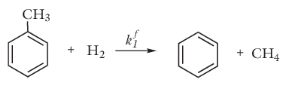
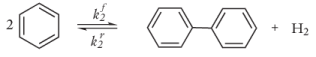
PDF

Hydrodealkylation in a Membrane Reactor
Introduction
At high temperatures and pressures, and in the presence of hydrogen, toluene can be demethylated to produce benzene. Furthermore, benzene can react reversibly to produce biphenyl. The following example illustrates the simulation of the hydrodealkylation process, carried out in a membrane reactor. This reactor arrangement allows for continuous addition of hydrogen to the process, increasing the selectivity for the desired benzene product.
The example shows how you can easily modify the predefined Plug Flow reactor type in the Reaction Engineering interface to set up a membrane reactor model. We will also learn how to create a Thermodynamic System from Thermodynamics to get different thermodynamic and physical property functions for each compound and their mixture. After all species in Reaction Engineering have been coupled to a corresponding species in the Thermodynamic system, the required species and mixture properties will automatically be created and added to the package.
Model Definition
Two important reactions occur in the thermal hydrodealkylation (HDA) of toluene. The main reaction involves toluene reacting with hydrogen to produce benzene and methane:
(1)
The dealkylation reaction rate is first order in the toluene concentration and half order in the hydrogen concentration:
At the same time, biphenyl is reversibly formed from benzene:
(2)
The rate of the coupling reaction follows the mass action law:
In the above rate expressions, the rate constants follow Arrhenius type behavior:
The values of the frequency factors and activation energies (J/mol) are taken from the literature (Ref. 1 and Ref. 2) and are presented in Table 1.
The chemical reactions given in Equation 1 and Equation 2 suggest that maintaining high concentrations of hydrogen would be beneficial to ensure a high benzene yield. Such process conditions can be achieved by using a membrane reactor. As illustrated schematically in Figure 1, hydrogen can be supplied continuously across the porous membrane.
Figure 1: Hydrogen is continuously supplied to the reactor through a porous membrane.
The species mass balance for hydrogen in the membrane reactor is given by:
where F is the molar flow rate (SI unit: mol/s) in the reactor, V is the reactor volume (SI unit: m3), R is the species rate expression (SI unit: mol/(m3·s)), and f is the molar flow rate per unit volume (SI unit: mol/(m3·s)) across the membrane. The velocity of the hydrogen gas across the porous membrane can be described by Darcy’s law:
where K (SI unit: m3/(N·s)) is a proportionality constant, pshell (SI unit: Pa) is the gas pressure on the shell side of the membrane, and preactor (SI unit: Pa) the pressure on the reactor side. The molar flow rate per unit volume across the membrane then becomes:
Above, a is the membrane surface area per unit volume (SI unit: m2/m3), and cshell is the concentration of hydrogen (SI unit: mol/m3) on the shell side.
Except for hydrogen, the other chemical species in the reactor do not pass through the membrane and their material balances thus follow the standard plug flow equations:
(3)
The adiabatic energy balance for the reactor is given by:
(4)
In Equation 4, Cmix represents the mixture (reacting system) molar heat capacity (SI unit: J/(mol·K)), and Q denotes the heat due to chemical reaction (SI unit: J/(m3·s)):
where Hj is the heat produced by reaction j, calculated from:
(5)
In Equation 5 hi represents the species partial molar enthalpy (SI unit: J/mol) and νij the stoichiometric coefficients.
The last term in the energy balance accounts for the energy transfer associated with the flow of hydrogen across the membrane:
The Reaction Engineering interface automatically sets up and solves Equation 3 and Equation 4 when you select the predefined Plug-flow reactor type. To adjust the default model to account for hydrogen entering the reactor through the membrane, the flow term fH has to be specified and included into the hydrogen material balance.
Solving the energy balance, Equation 4, requires the input of mixture molar heat capacities Cmix (SI unit: J/(mol·K)), and the partial molar enthalpies, hi (SI unit: J/mol), of the reacting species. In this example, these thermodynamic properties are calculated from the thermodynamic system.
Results and Discussion
In a first simulation, the reactor is assumed to be a standard tubular reactor, that is, without hydrogen entering through the reactor circumference. The reactor is fed with equal molar flows (10 mol/s) of hydrogen and toluene. At the inlet the reactant gas is held at 1200 K and 2 atmospheres. The result is shown in Figure 2.
Figure 2: Concentration (mol/m3) and temperature (K) as function of reactor volume (m3) for a tubular reactor design.
A second model simulates the membrane reactor, with a continuous supply of hydrogen through the membrane. Figure 3 shows the corresponding concentration distributions.
Figure 3: Concentration (mol/m3) and temperature (K) as function of reactor volume (m3) for a membrane reactor design with a continuous supply of hydrogen.
The biphenyl concentration is reduced versus that obtained from the first model. Clearly, the membrane reactor produces benzene with greater selectivity. However, note that this comparison is somewhat lacking in this particular model, the total amount of added hydrogen differs due to the flow across the membrane being an additional source. A more elaborate model, with irreversible reactions leading to unwanted byproducts, would however exhibit differences even after compensating for different amounts of hydrogen.
References
1. K.C. Hou and H.B. Palmer, “The Kinetics of Thermal Decomposition of Benzene in a Flow System,” J. Phys. Chem., vol. 69, no. 3, pp. 863–868, 1965.
2. S.E. Shull and A.N. Hixson, I&EC Process Design and Development, vol. 5, p. 147, 1966.
Application Library path: Chemical_Reaction_Engineering_Module/Thermodynamics/membrane_hda
Note: This model is included in the booklet Introduction to Thermodynamic Properties.
Modeling Instructions
From the File menu, choose New.
New
In the New window, click  Model Wizard.
Model Wizard
1
In the Model Wizard window, click  0D.
2
In the Select Physics tree, select Chemical Species Transport > Reaction Engineering (re).
3
Click Add.
4
Click  Study.
5
In the Select Study tree, select Preset Studies for Selected Physics Interfaces > Stationary Plug Flow.
6
Reaction Engineering (re)
In this model, a Thermodynamic System will be created from Thermodynamics. The Thermodynamic System includes all thermodynamic properties (such as enthalpy, entropy, etc) which are needed in the simulation of reacting system. The properties from Thermodynamics are coupled to Reaction Engineering automatically.
1
In the Reaction Engineering toolbar, click  Thermodynamics and choose Thermodynamic System.
First, select a phase state for the Thermodynamic System.
Select System
1
Go to the Select System window.
Select phases Vapor-liquid.
2
From the Phase list, choose Vapor–liquid.
3
Click the Next button in the window toolbar.
Select species hydrogen, methane, benzene, toluene and biphenyl.
Select Species
1
Go to the Select Species window.
2
In the Species list box, select hydrogen (1333-74-0, H2).
3
Click  Add Selected.
4
In the Species list box, select methane (74-82-8, CH4).
5
Click  Add Selected.
6
In the Species list box, select benzene (71-43-2, C6H6).
7
Click  Add Selected.
8
In the Species list box, select toluene (108-88-3, C7H8).
9
Click  Add Selected.
10
In the Species list box, select biphenyl (92-52-4, C12H10).
11
Click  Add Selected.
12
Click the Next button in the window toolbar.
Select Thermodynamic Model
1
Go to the Select Thermodynamic Model window.
2
Click the Finish button in the window toolbar.
Global Definitions
Vapor–Liquid System 1 (pp1)
Create a mixture function for enthalpy of formation to introduce a heat source used later in Reaction Engineering.
1
Right-click Global Definitions > Thermodynamics > Vapor–Liquid System 1 (pp1) and choose Mixture Property.
Select Properties
1
Go to the Select Properties window.
2
In the list box, select Enthalpy of formation (J/mol).
3
Click  Add Selected.
4
Click the Next button in the window toolbar.
Select Phase
1
Go to the Select Phase window.
2
Click the Next button in the window toolbar.
Select Species
1
Go to the Select Species window.
2
Click  Add All.
3
Click the Next button in the window toolbar.
Mixture Property Overview
1
Go to the Mixture Property Overview window.
2
Click the Finish button in the window toolbar.
Global Definitions
Enthalpy of formation 1 (EnthalpyF_benzene_biphenyl_hydrogen_methane_toluene_Vapor11, EnthalpyF_benzene_biphenyl_hydrogen_methane_toluene_Vapor11_Dtemperature, EnthalpyF_benzene_biphenyl_hydrogen_methane_toluene_Vapor11_Dpressure)
Change the function name to hF_mixture.
1
In the Settings window for Mixture Property, type hF_mixture in the Function name text field.
Load model parameters by importing their definitions from a text file.
Parameters 1
1
In the Model Builder window, under Global Definitions click Parameters 1.
2
In the Settings window for Parameters, locate the Parameters section.
3
Click  Load from File.
4
Definitions
Add variable definitions from a text file.
Variables 1
1
In the Model Builder window, under Component 1 (comp1) right-click Definitions and choose Variables.
2
In the Settings window for Variables, locate the Variables section.
3
Click  Load from File.
4
Note that some expressions use functions in Thermodynamics and variables defined in the Reaction Engineering interface. These variables need to be specified with the scope of the Reaction Engineering node. For example, re.T specifies the temperature variable defined by the Reaction Engineering node with the identifier re.
Reaction Engineering (re)
1
In the Model Builder window, under Component 1 (comp1) click Reaction Engineering (re).
2
In the Settings window for Reaction Engineering, locate the Reactor section.
3
From the Reactor type list, choose Plug flow.
4
Locate the Energy Balance section. From the Energy balance list, choose Include.
5
In the Q text field, type Q_mem.
This accounts for the heat transferred into the reactor due to the flow across the membrane.
6
Click to expand the Mixture Properties section. In the p text field, type p_reactor.
Reaction 1
1
In the Reaction Engineering toolbar, click  Reaction.
2
In the Settings window for Reaction, locate the Reaction Formula section.
3
In the Formula text field, type C6H5CH3+H2=>C6H6+CH4.
4
Locate the Rate Constants section. Select the Use Arrhenius expressions checkbox.
5
In the Af text field, type 5.67e9[1/s].
6
In the Ef text field, type 228.2e3.
7
Locate the Reaction Rate section. From the list, choose User defined.
8
Locate the Reaction Orders section. Find the Volumetric overall reaction order subsection. In the Forward text field, type 1.
9
Locate the Reaction Rate section. In the rj text field, type re.kf_1*re.c_C6H5CH3*(re.c_H2/1[mol/m^3])^0.5.
Change the default kinetic expression by modifying the reaction order for hydrogen.
Reaction 2
1
In the Reaction Engineering toolbar, click  Reaction.
2
In the Settings window for Reaction, locate the Reaction Formula section.
3
In the Formula text field, type 2C6H6<=>C12H10+H2.
4
Locate the Rate Constants section. Select the Use Arrhenius expressions checkbox.
5
In the Af text field, type 1e8.
6
In the Ef text field, type 167.5e3.
7
In the Ar text field, type 1e8.
8
In the Er text field, type 149.8e3.
Additional Source 1
You will now add an Additional Source feature to Reaction Engineering to the membrane reactor model.
1
In the Reaction Engineering toolbar, click  Additional Source.
2
In the Settings window for Additional Source, locate the Additional Rate Expression section.
3
In the Volumetric species table, enter the following settings:
The f_H2 term corresponds to the flow of hydrogen across the membrane.
Initial Values 1
The plug flow reactor requires you to input the inlet molar flow.
1
In the Model Builder window, click Initial Values 1.
2
In the Settings window for Initial Values, locate the General Parameters section.
3
In the T0,in text field, type T_inlet.
4
Locate the Volumetric Species Initial Values section. In the table, enter the following settings:
Couple all species in Reaction Engineering to corresponding species in the created Thermodynamic System. For a coupled species, its thermodynamic properties will be set automatically to the coupled Thermodynamic System. When all species in Reaction Engineering are coupled (fully coupled), the properties of the reacting system (heat capacity, molar volume, etc) will be calculated from the Thermodynamic System.
5
In the Model Builder window, click Reaction Engineering (re).
6
In the Settings window for Reaction Engineering, locate the Mixture Properties section.
7
Select the Thermodynamics checkbox.
8
Locate the Species Matching section. In the table, enter the following settings:
In the present example the total reactor volume is 1 m3, so default solver settings can be used.
Tubular reactor
You have now set up a model for a nonisothermal tubular reactor. For the tubular reactor, the Additional Source feature is disabled. First solve this model and review the results, then move on to study the related membrane reactor model with the Additional Source feature.
1
In the Model Builder window, right-click Study 1 and choose Rename.
2
In the Rename Study dialog, type Tubular reactor in the New label text field.
3
Step 1: Stationary Plug Flow
1
In the Model Builder window, under Tubular reactor click Step 1: Stationary Plug Flow.
2
In the Settings window for Stationary Plug Flow, locate the Physics and Variables Selection section.
3
Select the Modify model configuration for study step checkbox.
4
In the tree, select Component 1 (comp1) > Reaction Engineering (re) > Additional Source 1.
5
6
In the Model Builder window, click Tubular reactor.
7
In the Settings window for Study, locate the Study Settings section.
8
Clear the Generate default plots checkbox.
9
In the Study toolbar, click  Compute.
Results
1D Plot Group 1
In the Results toolbar, click  1D Plot Group.
Global 1
Right-click 1D Plot Group 1 and choose Global.
Global 2
In the Model Builder window, right-click 1D Plot Group 1 and choose Global.
Concentration and Temperature profile, tubular reactor
1
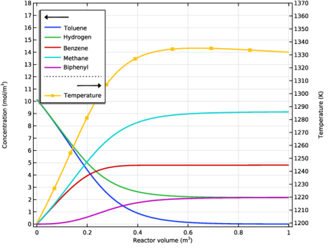
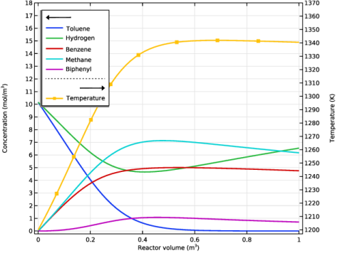
In the Settings window for 1D Plot Group, type Concentration and Temperature profile, tubular reactor in the Label text field.
2
Locate the Plot Settings section.
3
Select the x-axis label checkbox. In the associated text field, type Reactor volume (m<sup>3</sup>).
4
Select the y-axis label checkbox. In the associated text field, type Concentration (mol/m<sup>3</sup>).
5
Select the Two y-axes checkbox.
6
In the table, select the Plot on secondary y-axis checkbox for Global 2.
7
Select the Secondary y-axis label checkbox. In the associated text field, type Temperature (K).
Concentration
1
In the Model Builder window, under Results > Concentration and Temperature profile, tubular reactor click Global 1.
2
In the Settings window for Global, type Concentration in the Label text field.
3
Locate the y-Axis Data section. In the table, enter the following settings:
4
Click to expand the Legends section. From the Legends list, choose Manual.
5
6
Click to expand the Coloring and Style section. From the Width list, choose 2.
Temperature
1
In the Model Builder window, under Results > Concentration and Temperature profile, tubular reactor click Global 2.
2
In the Settings window for Global, type Temperature in the Label text field.
3
Locate the y-Axis Data section. Click  Clear Table.
4
5
Locate the Coloring and Style section. From the Width list, choose 2.
6
Find the Line markers subsection. From the Marker list, choose Point.
7
From the Positioning list, choose Interpolated.
8
In the Concentration and Temperature profile, tubular reactor toolbar, click  Plot.
9
10
Locate the Legends section. Find the Include subsection. Select the Label checkbox.
11
Clear the Solution checkbox.
12
Clear the Expression checkbox.
Concentration and Temperature profile, tubular reactor
1
In the Model Builder window, click Concentration and Temperature profile, tubular reactor.
2
In the Settings window for 1D Plot Group, click to expand the Title section.
3
From the Title type list, choose None.
4
Locate the Axis section. Select the Manual axis limits checkbox.
5
In the y maximum text field, type 18.
6
In the Secondary y maximum text field, type 1370.
7
Locate the Legend section. From the Position list, choose Upper left.
8
In the Concentration and Temperature profile, tubular reactor toolbar, click  Plot.
Add Study
1
In the Home toolbar, click  Add Study to open the Add Study window.
2
Go to the Add Study window.
3
Find the Studies subsection. In the Select Study tree, select Preset Studies for Selected Physics Interfaces > Stationary Plug Flow.
4
Click the Add Study button in the window toolbar.
5
In the Home toolbar, click  Add Study to close the Add Study window.
Membrane reactor
1
In the Settings window for Study, type Membrane reactor in the Label text field.
Note: the Additional Source feature is included in membrane reactor model.
2
Locate the Study Settings section. Clear the Generate default plots checkbox.
3
In the Study toolbar, click  Compute.
Results
Concentration and Temperature profile, membrane reactor
1
Right-click Concentration and Temperature profile, tubular reactor and choose Duplicate.
2
In the Settings window for 1D Plot Group, type Concentration and Temperature profile, membrane reactor in the Label text field.
3
Locate the Data section. From the Dataset list, choose Membrane reactor/Solution 2 (sol2).
4
In the Concentration and Temperature profile, membrane reactor toolbar, click  Plot.