





PDF

Boat Reactor for Low-Pressure Chemical Vapor Deposition
Introduction
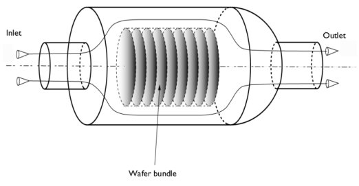
Chemical vapor deposition (CVD) is an important step in the process of manufacturing microchips. A common application is the deposition of silicon on wafers at low pressure. Low-pressure reactors such as shown in Figure 1 below are used to get a high diffusivity of the gaseous species, which results in a uniform deposition thickness, because the process becomes limited by the deposition kinetics (Ref. 1 and Ref. 2).
Figure 1: Schematic of a boat reactor and principle of the deposition process.
The gas, in this case silane (SiH4), enters the reactor from the left and reacts on the wafers to form hydrogen and silicon. The remaining mixture leaves the reactor through the outlet on the right. The deposition of silicon on the wafers surface depends on the silane concentration. Further details can be found in Elements of Chemical Reaction Engineering  by H. Scott Fogler (Ref. 1).
This example models the coupled reaction kinetics, fluid, and mass transport in a low-pressure boat reactor to describe the rate of deposition as a function of the operating conditions.
Model Definition
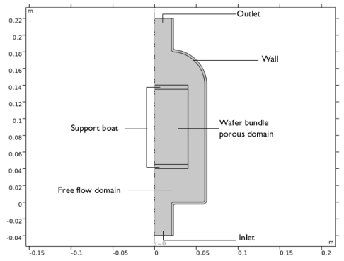
Figure 2 shows the modeled domain of the boat reactor which is simplified as a 2D axisymmetric geometry. To further simplify the geometry and to save computational memory, the wafer bundle is modeled as a porous medium. The temperature in the reactor is assumed to be constant.
Figure 2: Model geometry including the domain and boundary labels.
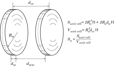
The specific surface area (m2/m3) of the wafer bundle porous medium is calculated as the area per volume by assuming a pitch between the wafers as seen in Figure 3 below.
Figure 3: Specific surface area of wafer bundle calculation.
The wafer bundle porosity is the wafer volume per bundle volume:
Chemistry
In the wafer bundle, silane gas reacts to form solid silicon which is deposited on the wafers:
The reaction rate, Ri (mol/(m3·s)), is expressed as a first order reaction as follows:
(1)
where cSiH4 is the local concentration (mol/m3) and k is the rate constant (m/s) which is based on experimental results (Ref. 2) as follows:
where a (m/s) and b (1/Pa) are experimental kinetic parameters (based on Ref. 2) which depend on temperature as follows:
where kB is the Boltzmann constant (J/K) and T is the reactor temperature (K).
A crucial characteristic of the reactor performance is the growth rate of the silicon layers on the wafers known as the deposition rate, ΔSi (m/s), which is calculated as follows:
where MSi is the molar mass (kg/mol) and ρSi is the density (kg/m3) of silicon.
The reacting gas species are diluted in inert nitrogen gas which is assumed to well represent the properties of the mixture.
Fluid Flow
The flow in the reactor is modeled as laminar fluid flow. Flow inside the wafer bundle is neglected such that the reacting gas are only be transported by diffusion. This is justified since only transport in the radial direction is permitted by the physical wafers. And only dilute gas species, silane and hydrogen, experience a net transport through the wafer bundle from the deposition process. The inlet velocity is assumed to be fully developed with an average velocity and there is no slip at the reactor walls, support boat and along the wafer bundle.
Mass transport
The diffusion, convection, and reaction of each gaseous species i in the diluted solution is described as follows:
where Di is diffusion coefficient (m2/s), ci is the concentration (mol/m3), u is the velocity vector (m/s), and  Ri is the reaction rate (mol/(m3·s)), as defined in Equation 1. The reaction is defined only in the wafer bundle domain and therefore the reaction rate term is zero in the free flow domain. Since the gases do not diffuse through the physical wafers, the axial diffusion in the porous medium representing the wafer bundle is neglected by setting the z-component of the diffusivity matrix to zero. The inlet concentration of silane is defined from the ideal gas law at the operating conditions and there is no mass flux perpendicular to the support boat or the reactor wall boundaries.
Results and Discussion
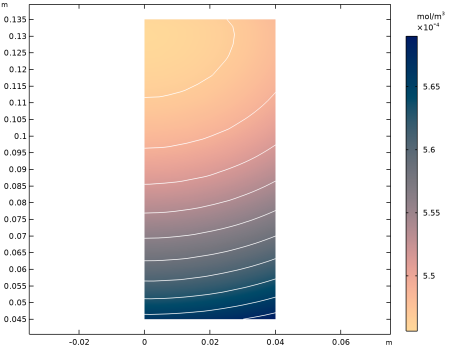
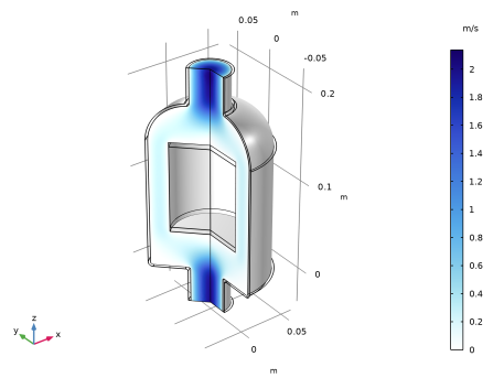
Figure 4 shows the velocity profile in the reactor, indicating that the velocity in the wafer bundle is much smaller than in the free flowing domain. Figure 5 shows the concentration profile in the wafer bundle of the silane gas, which dictates the deposition rate and thickness of silicon.
Figure 4: Velocity profile in boat reactor 600°C, 25 Pa.
Figure 5: Silane concentration profile in wafer bundle at 600°C, 25 Pa. Lines indicate the concentration isocontours.
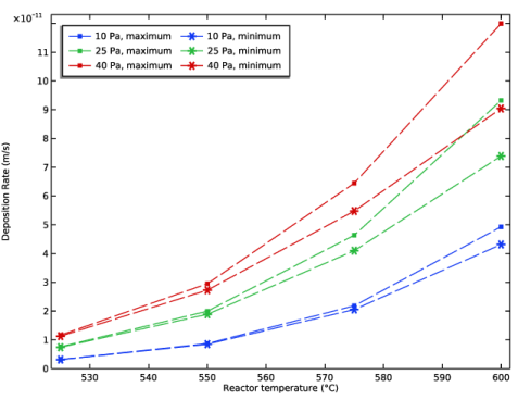
Figure 5 shows the concentration of the silane in the wafer bundle which is used to estimate the deposition rate of silicon on the wafers as shown in Figure 6 below. The highest concentration of silane is obtained near the reactor inlet and close to the free-fluid channel. The relative variation in silane concentration over the wafer bundle domain is 3.6%.
Figure 6: Variation in deposition rate with temperature, total pressure, and location in wafer bundle. The asterisks represent the minimum expected deposition rate whereas the squares represent the maximum expected deposition rate in the wafer bundle. The colors of the lines represent operating pressures.
Figure 6 shows that the variation in the deposition rate of silicon increases as the operating temperature and pressure of the reactor increases. Therefore, operating at lower pressures and higher temperatures is favorable to ensure a uniform deposition rate over the wafer bundle due to the higher diffusivity of the gaseous species.
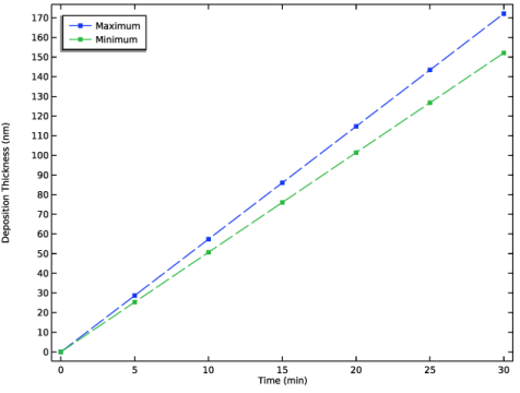
Figure 7: Deposition thickness over time at 575°C, 25 Pa.
References
1. H. Scott Fogler, Elements of Chemical Reaction Engineering, 3rd ed., Prentice Hall, 1999.
2. A.T. Voutsas and M.K. Hatalis, “Structure of As-Deposited LPCVD Silicon Films at Low Deposition Temperatures and Pressures,” J. Electrochem. Soc., vol. 139, no. 9, pp. 2659–2665, 1992.
Application Library path: Chemical_Reaction_Engineering_Module/Reactors_with_Mass_Transfer/boat_reactor
Modeling Instructions
From the File menu, choose New.
New
In the New window, click  Model Wizard.
Model Wizard
1
In the Model Wizard window, click  2D Axisymmetric.
2
In the Select Physics tree, select Chemical Species Transport > Chemistry (chem).
3
Click Add.
4
In the Select Physics tree, select Fluid Flow > Single-Phase Flow > Laminar Flow (spf).
5
Click Add.
6
In the Select Physics tree, select Chemical Species Transport > Transport of Diluted Species (tds).
7
Click Add.
8
Click  Add Concentration.
9
In the Concentrations (mol/m³) table, enter the following settings:
10
Click  Study.
11
In the Select Study tree, select General Studies > Stationary.
12
Global Definitions
Add the model parameters by importing their definitions from a data text file provided with the Application Library.
Geometric Parameters
1
In the Home toolbar, click  Parameters and choose Select > Parameters 1.
2
In the Settings window for Parameters, type Geometric Parameters in the Label text field.
3
Locate the Parameters section. Click  Load from File.
4
Operating Parameters
1
In the Home toolbar, click  Parameters and choose Add > Parameters.
2
In the Settings window for Parameters, type Operating Parameters in the Label text field.
3
Locate the Parameters section. Click  Load from File.
4
First, build the reactor geometry.
Geometry 1
Reactor
1
In the Model Builder window, under Component 1 (comp1) right-click Geometry 1 and choose Node Group.
2
In the Settings window for Group, type Reactor in the Label text field.
Rectangle 1 (r1)
1
In the Geometry toolbar, click  Rectangle.
2
In the Settings window for Rectangle, locate the Size and Shape section.
3
In the Width text field, type W.
4
In the Height text field, type L.
5
Click  Build Selected.
Fillet 1 (fil1)
1
In the Geometry toolbar, click  Fillet.
2
On the object r1, select Point 3 only.
3
In the Settings window for Fillet, locate the Radius section.
4
In the Radius text field, type R_curve.
5
Click  Build Selected.
Rectangle 2 (r2)
1
In the Geometry toolbar, click  Rectangle.
2
In the Settings window for Rectangle, locate the Size and Shape section.
3
In the Width text field, type R_tube.
4
In the Height text field, type L_tube.
5
Locate the Position section. In the z text field, type -L_tube.
6
Click  Build Selected.
Rectangle 3 (r3)
1
In the Geometry toolbar, click  Rectangle.
2
In the Settings window for Rectangle, locate the Size and Shape section.
3
In the Width text field, type R_tube.
4
In the Height text field, type L_tube.
5
Locate the Position section. In the z text field, type L.
6
Click  Build Selected.
Union 1 (uni1)
1
In the Geometry toolbar, click  Booleans and Partitions and choose Union.
2
Click in the Graphics window and then press Ctrl+A to select all objects.
3
In the Settings window for Union, locate the Union section.
4
Clear the Keep interior boundaries checkbox.
5
Click  Build Selected.
Fillet 2 (fil2)
1
In the Geometry toolbar, click  Fillet.
2
On the object uni1, select Points 6, 7, and 9 only.
3
In the Settings window for Fillet, locate the Radius section.
4
In the Radius text field, type b.
5
Click  Build Selected.
Thicken 1 (thi1)
1
In the Geometry toolbar, click  Conversions and choose Thicken.
2
In the Settings window for Thicken, locate the Input section.
3
From the Geometric entity level list, choose Boundary.
4
On the object fil2, select Boundaries 6–13 only.
5
Select the Keep input objects checkbox.
6
Locate the Options section. From the Offset list, choose Asymmetric.
7
In the Upside thickness text field, type b.
8
Click  Build Selected.
Fillet 3 (fil3)
1
In the Geometry toolbar, click  Fillet.
2
On the object thi1, select Points 7 and 9 only.
3
In the Settings window for Fillet, locate the Radius section.
4
In the Radius text field, type b.
5
Click  Build Selected.
Wafer Bundle
1
In the Model Builder window, right-click Geometry 1 and choose Node Group.
Next, build the wafer bundle geometry.
2
In the Settings window for Group, type Wafer Bundle in the Label text field.
Rectangle 4 (r4)
1
In the Geometry toolbar, click  Rectangle.
2
In the Settings window for Rectangle, locate the Size and Shape section.
3
In the Width text field, type R_w.
4
In the Height text field, type L_wb.
5
Locate the Position section. In the z text field, type L_space.
6
Click  Build Selected.
Rectangle 5 (r5)
1
In the Geometry toolbar, click  Rectangle.
2
In the Settings window for Rectangle, locate the Size and Shape section.
3
In the Width text field, type R_w.
4
In the Height text field, type H_sb.
5
Locate the Position section. In the z text field, type L_space.
6
Click  Build Selected.
Rectangle 6 (r6)
1
In the Geometry toolbar, click  Rectangle.
2
In the Settings window for Rectangle, locate the Size and Shape section.
3
In the Width text field, type R_w.
4
In the Height text field, type H_sb.
5
Locate the Position section. In the z text field, type L_space+L_wb-H_sb.
6
Click  Build Selected.
Form Union (fin)
1
In the Model Builder window, under Component 1 (comp1) > Geometry 1 click Form Union (fin).
2
In the Settings window for Form Union/Assembly, click  Build Selected.
3
Click the  Zoom Extents button in the Graphics toolbar.
Definitions
Next, define explicit selections with descriptive names for three domains to facilitate making selections in the physics interfaces later.
Wafer Bundle
1
In the Definitions toolbar, click  Explicit.
2
3
In the Settings window for Explicit, type Wafer Bundle in the Label text field.
Reactor
1
In the Definitions toolbar, click  Explicit.
2
3
In the Settings window for Explicit, type Reactor in the Label text field.
Wall
1
In the Definitions toolbar, click  Explicit.
2
3
In the Settings window for Explicit, type Wall in the Label text field.
Variables 1
1
In the Definitions toolbar, click  Local Variables.
2
In the Settings window for Variables, locate the Variables section.
3
Chemistry (chem)
1
In the Model Builder window, under Component 1 (comp1) click Chemistry (chem).
2
In the Settings window for Chemistry, locate the Model Input section.
3
From the T list, choose User defined. In the associated text field, type T_r.
4
From the p list, choose User defined. In the associated text field, type p_tot.
Reaction 1
1
In the Physics toolbar, click  Domains and choose Reaction.
2
In the Settings window for Reaction, locate the Reaction Formula section.
3
In the Formula text field, type SiH4 => Si(s) + 2 H2.
4
Click Apply.
5
Locate the Rate Constants section. In the kf text field, type k_rxn*S_a.
Species 1
1
In the Physics toolbar, click  Domains and choose Species.
2
In the Settings window for Species, locate the Name section.
3
4
Locate the Type section. From the list, choose Solvent.
5
In the Model Builder window, click Chemistry (chem).
6
In the Settings window for Chemistry, locate the Species Matching section.
7
Find the Bulk species subsection. From the Species solved for list, choose Transport of Diluted Species.
8
9
Find the Solid species subsection. In the table, enter the following settings:
Laminar Flow (spf)
1
In the Model Builder window, under Component 1 (comp1) click Laminar Flow (spf).
2
3
In the Settings window for Laminar Flow, locate the Physical Model section.
4
In the pref text field, type p_tot.
5
In the Tref text field, type T_r.
Fluid Properties 1
1
In the Model Builder window, under Component 1 (comp1) > Laminar Flow (spf) click Fluid Properties 1.
2
In the Settings window for Fluid Properties, locate the Fluid Properties section.
3
From the ρ list, choose Density (chem).
4
From the μ list, choose Dynamic viscosity (chem).
Inlet 1
1
In the Physics toolbar, click  Boundaries and choose Inlet.
2
3
In the Settings window for Inlet, locate the Boundary Condition section.
4
From the list, choose Fully developed flow.
5
Locate the Fully Developed Flow section. In the Uav text field, type v0.
Outlet 1
1
In the Physics toolbar, click  Boundaries and choose Outlet.
2
Transport of Diluted Species (tds)
1
In the Model Builder window, under Component 1 (comp1) click Transport of Diluted Species (tds).
2
In the Settings window for Transport of Diluted Species, locate the Domain Selection section.
3
From the Selection list, choose Reactor.
4
Locate the Transport Mechanisms section. Select the Mass transfer in porous media checkbox.
Fluid 1
1
In the Model Builder window, under Component 1 (comp1) > Transport of Diluted Species (tds) click Fluid 1.
2
In the Settings window for Fluid, locate the Model Input section.
3
From the T list, choose User defined. In the associated text field, type T_r.
4
Locate the Convection section. From the u list, choose Velocity field (spf).
5
Locate the Diffusion section. From the Source list, choose Chemistry.
6
From the DcSiH4 list, choose Diffusion coefficient , SiH4 in N2 (solvent) (chem).
7
From the DcH2 list, choose Diffusion coefficient , H2 in N2 (solvent) (chem).
Reactions 1
1
In the Physics toolbar, click  Domains and choose Reactions.
2
In the Settings window for Reactions, locate the Domain Selection section.
3
From the Selection list, choose Wafer Bundle.
4
Locate the Reaction Rates section. From the Chemistry list, choose Chemistry (chem).
5
Locate the Reacting Volume section. From the list, choose Pore volume.
Inflow 1
1
In the Physics toolbar, click  Boundaries and choose Inflow.
2
3
In the Settings window for Inflow, locate the Concentration section.
4
In the c0,cSiH4 text field, type c_SiH4.
Outflow 1
1
In the Physics toolbar, click  Boundaries and choose Outflow.
2
Porous Medium 1
1
In the Physics toolbar, click  Domains and choose Porous Medium.
2
In the Settings window for Porous Medium, locate the Domain Selection section.
3
From the Selection list, choose Wafer Bundle.
Fluid 1
1
In the Model Builder window, click Fluid 1.
2
In the Settings window for Fluid, locate the Model Input section.
3
From the T list, choose User defined. In the associated text field, type T_r.
4
Locate the Convection section. From the u list, choose Velocity field (spf).
5
Locate the Diffusion section. From the Source list, choose Chemistry.
6
7
Specify the DcSiH4 matrix as
8
9
Specify the DcH2 matrix as
10
From the Effective diffusivity model list, choose No correction.
Porous Matrix 1
1
In the Model Builder window, click Porous Matrix 1.
2
In the Settings window for Porous Matrix, locate the Matrix Properties section.
3
From the εp list, choose User defined. In the associated text field, type e_p.
Multiphysics
Reacting Flow, Diluted Species 1 (rfd1)
In the Physics toolbar, click  Multiphysics Couplings and choose Domain > Reacting Flow, Diluted Species.
Mesh 1
In the Model Builder window, under Component 1 (comp1) right-click Mesh 1 and choose Build All.
Study 1
Parametric Sweep
1
In the Study toolbar, click  Parametric Sweep.
2
In the Settings window for Parametric Sweep, locate the Study Settings section.
3
From the Sweep type list, choose All combinations.
4
5
6
7
In the Study toolbar, click  Compute.
Results
Velocity (spf)
1
In the Settings window for 2D Plot Group, locate the Data section.
2
From the Parameter value (p_tot (Pa)) list, choose 25.
3
Click to expand the Title section. From the Title type list, choose None.
4
Locate the Color Legend section. Select the Show units checkbox.
Surface
1
In the Model Builder window, expand the Velocity (spf) node, then click Surface.
2
In the Settings window for Surface, locate the Coloring and Style section.
3
From the Color table list, choose Kyanite.
Pressure (spf)
1
In the Model Builder window, under Results click Pressure (spf).
2
In the Settings window for 2D Plot Group, locate the Data section.
3
From the Parameter value (p_tot (Pa)) list, choose 25.
4
Locate the Title section. From the Title type list, choose None.
5
Locate the Color Legend section. Select the Show units checkbox.
Surface 1
1
In the Model Builder window, expand the Pressure (spf) node, then click Surface 1.
2
In the Settings window for Surface, locate the Coloring and Style section.
3
From the Color table list, choose Kyanite.
Velocity, 3D (spf)
1
In the Model Builder window, under Results click Velocity, 3D (spf).
2
In the Settings window for 3D Plot Group, locate the Data section.
3
From the Parameter value (p_tot (Pa)) list, choose 25.
4
Click to expand the Title section. From the Title type list, choose None.
5
Locate the Color Legend section. Select the Show units checkbox.
Surface
1
In the Model Builder window, expand the Velocity, 3D (spf) node, then click Surface.
2
In the Settings window for Surface, locate the Coloring and Style section.
3
From the Color table list, choose Kyanite.
4
Click the  Zoom Extents button in the Graphics toolbar.
Concentration, SiH4 (tds)
1
In the Model Builder window, under Results click Concentration, SiH4 (tds).
2
In the Settings window for 2D Plot Group, locate the Data section.
3
From the Parameter value (p_tot (Pa)) list, choose 25.
4
Locate the Title section. From the Title type list, choose None.
5
Locate the Color Legend section. Select the Show units checkbox.
Surface 1
1
In the Model Builder window, expand the Concentration, SiH4 (tds) node, then click Surface 1.
2
In the Settings window for Surface, locate the Coloring and Style section.
3
From the Color table list, choose Agama.
4
Click the  Zoom Extents button in the Graphics toolbar.
Concentration, SiH4 (tds) 1
1
In the Model Builder window, right-click Concentration, SiH4 (tds) and choose Duplicate.
2
Drag and drop Concentration, SiH4 (tds) 1 below Concentration, SiH4 (tds).
Surface 1
In the Model Builder window, expand the Concentration, SiH4 (tds) 1 node, then click Surface 1.
Selection 1
1
In the Concentration, SiH4 (tds) 1 toolbar, click  Selection.
2
In the Settings window for Selection, locate the Selection section.
3
From the Selection list, choose Wafer Bundle.
Arrow Surface 1
In the Model Builder window, under Results > Concentration, SiH4 (tds) 1 right-click Arrow Surface 1 and choose Disable.
Surface 1
In the Model Builder window, click Surface 1.
Concentration, SiH4 (tds) 1
In the Concentration, SiH4 (tds) 1 toolbar, click  Contour.
Contour 1
1
In the Settings window for Contour, locate the Expression section.
2
In the Expression text field, type cSiH4.
3
Click to expand the Title section. From the Title type list, choose None.
4
Locate the Levels section. In the Total levels text field, type 10.
5
Locate the Coloring and Style section. From the Coloring list, choose Uniform.
6
From the Color list, choose White.
7
Clear the Color legend checkbox.
Selection 1
1
In the Concentration, SiH4 (tds) 1 toolbar, click  Selection.
2
In the Settings window for Selection, locate the Selection section.
3
From the Selection list, choose Wafer Bundle.
Concentration, SiH4 (tds) 1
1
In the Model Builder window, under Results click Concentration, SiH4 (tds) 1.
2
In the Settings window for 2D Plot Group, locate the Plot Settings section.
3
Clear the Plot dataset edges checkbox.
4
In the Concentration, SiH4 (tds) 1 toolbar, click  Plot.
5
Click the  Zoom Extents button in the Graphics toolbar.
Concentration, SiH4, 3D (tds)
1
In the Model Builder window, click Concentration, SiH4, 3D (tds).
2
In the Settings window for 3D Plot Group, locate the Data section.
3
From the Parameter value (p_tot (Pa)) list, choose 25.
4
Locate the Title section. From the Title type list, choose None.
5
Locate the Color Legend section. Select the Show units checkbox.
Surface 1
1
In the Model Builder window, expand the Concentration, SiH4, 3D (tds) node, then click Surface 1.
2
In the Settings window for Surface, locate the Coloring and Style section.
3
From the Color table list, choose Agama.
Concentration, H2 (tds)
1
In the Model Builder window, under Results click Concentration, H2 (tds).
2
In the Settings window for 2D Plot Group, locate the Data section.
3
From the Parameter value (p_tot (Pa)) list, choose 25.
4
Locate the Title section. From the Title type list, choose None.
5
Locate the Color Legend section. Select the Show units checkbox.
Surface 1
1
In the Model Builder window, expand the Concentration, H2 (tds) node, then click Surface 1.
2
In the Settings window for Surface, locate the Coloring and Style section.
3
From the Color table list, choose Caissara.
Concentration, H2, 3D (tds)
1
In the Model Builder window, under Results click Concentration, H2, 3D (tds).
2
In the Settings window for 3D Plot Group, locate the Data section.
3
From the Parameter value (p_tot (Pa)) list, choose 25.
4
Locate the Title section. From the Title type list, choose None.
5
Locate the Color Legend section. Select the Show units checkbox.
Surface 1
1
In the Model Builder window, expand the Concentration, H2, 3D (tds) node, then click Surface 1.
2
In the Settings window for Surface, locate the Coloring and Style section.
3
From the Color table list, choose Caissara.
Define a cut point at the center of the wafer bundle to study the deposition rate of silicon at this point as a function of operating conditions.
Midpoint
1
In the Results toolbar, click  Cut Point 2D.
2
In the Settings window for Cut Point 2D, locate the Point Data section.
3
In the r text field, type 0.
4
In the z text field, type L/2.
5
In the Label text field, type Midpoint.
6
Deposition rate vs T, P at midpoint
1
In the Results toolbar, click  1D Plot Group.
2
In the Settings window for 1D Plot Group, type Deposition rate vs T, P at midpoint in the Label text field.
3
Locate the Data section. From the Dataset list, choose Midpoint.
4
Click to expand the Title section. From the Title type list, choose None.
5
Locate the Grid section. Clear the Show grid checkbox.
6
Locate the Legend section. From the Position list, choose Upper left.
Point Graph 1
1
In the Deposition rate vs T, P at midpoint toolbar, click  Point Graph.
2
In the Settings window for Point Graph, locate the y-Axis Data section.
3
In the Expression text field, type Delta_Si.
4
Select the Description checkbox.
5
Locate the x-Axis Data section. From the Axis source data list, choose T_r.
6
From the Parameter list, choose Expression.
7
In the Expression text field, type T_r.
8
From the Unit list, choose °C.
9
Select the Description checkbox.
10
Click to expand the Coloring and Style section. Find the Line style subsection. From the Line list, choose Dashed.
11
Find the Line markers subsection. From the Marker list, choose Point.
12
Click to expand the Legends section. Select the Show legends checkbox.
13
Find the Include subsection. Clear the Point checkbox.
14
Clear the Solution checkbox.
15
Find the Prefix and suffix subsection. In the Prefix text field, type eval(p_tot, Pa) Pa.
16
In the Deposition rate vs T, P at midpoint toolbar, click  Plot.
Follow these instructions to generate Figure 6 in the model documentation.
Maximum 1
In the Results toolbar, click  More Datasets and choose Evaluation > Maximum.
Minimum 1
In the Results toolbar, click  More Datasets and choose Evaluation > Minimum.
Variation in deposition rate
1
In the Results toolbar, click  1D Plot Group.
2
In the Settings window for 1D Plot Group, type Variation in deposition rate in the Label text field.
3
Locate the Data section. From the Dataset list, choose Maximum 1.
4
Locate the Title section. From the Title type list, choose None.
5
Locate the Grid section. Clear the Show grid checkbox.
6
Locate the Legend section. From the Layout list, choose Inside graph axis area.
7
From the Position list, choose Upper left.
8
In the Number of columns text field, type 2.
9
In the Maximum relative width text field, type 1.
Maximum
1
In the Variation in deposition rate toolbar, click  Point Graph.
2
In the Settings window for Point Graph, type Maximum in the Label text field.
3
Locate the Data section. From the Dataset list, choose Maximum 1.
4
Locate the y-Axis Data section. Select the Description checkbox.
5
In the Expression text field, type Delta_Si.
6
In the Description text field, type Deposition Rate.
7
Locate the x-Axis Data section. From the Axis source data list, choose T_r.
8
From the Parameter list, choose Expression.
9
In the Expression text field, type T_r.
10
From the Unit list, choose °C.
11
Locate the Coloring and Style section. Find the Line style subsection. From the Line list, choose Dashed.
12
Find the Line markers subsection. From the Marker list, choose Point.
13
Locate the Legends section. Select the Show legends checkbox.
14
Find the Include subsection. Clear the Point checkbox.
15
Clear the Solution checkbox.
16
Find the Prefix and suffix subsection. In the Prefix text field, type eval(p_tot, Pa) Pa.
17
In the Suffix text field, type , maximum.
Variation in deposition rate
In the Variation in deposition rate toolbar, click  Point Graph.
Minimum
1
In the Settings window for Point Graph, type Minimum in the Label text field.
2
Locate the Data section. From the Dataset list, choose Minimum 1.
3
Locate the y-Axis Data section. In the Expression text field, type Delta_Si.
4
Select the Description checkbox.
5
Locate the x-Axis Data section. From the Axis source data list, choose T_r.
6
From the Parameter list, choose Expression.
7
In the Expression text field, type T_r.
8
From the Unit list, choose °C.
9
Locate the Coloring and Style section. Find the Line style subsection. From the Line list, choose Dashed.
10
Find the Line markers subsection. From the Marker list, choose Asterisk.
11
Locate the Legends section. Select the Show legends checkbox.
12
Find the Include subsection. Clear the Point checkbox.
13
Clear the Solution checkbox.
14
Find the Prefix and suffix subsection. In the Prefix text field, type eval(p_tot, Pa) Pa.
15
In the Suffix text field, type , minimum.
16
Locate the Coloring and Style section. From the Color list, choose Cycle (reset).
17
In the Variation in deposition rate toolbar, click  Plot.
The time-dependency needs to be introduced in order to study the deposition thickness. Since the system reaches steady state almost immediately, save computational memory by using an empty time-dependent study. The values of the dependent variables not solved for in this study are taken from the initial stationary study for a specific parameter sweep combination of interest.
Add Study
1
In the Study toolbar, click  Add Study to open the Add Study window.
2
Go to the Add Study window.
3
Find the Studies subsection. In the Select Study tree, select General Studies > Time Dependent.
4
Click the Add Study button in the window toolbar.
Study 2
Step 1: Time Dependent
1
In the Settings window for Time Dependent, locate the Study Settings section.
2
From the Time unit list, choose min.
3
In the Output times text field, type range(0,5,30).
4
Locate the Physics and Variables Selection section. In the Solve for column of the table, clear the checkbox for Component 1 (comp1).
5
Click to expand the Values of Dependent Variables section. Find the Values of variables not solved for subsection. From the Settings list, choose User controlled.
6
From the Method list, choose Solution.
7
From the Study list, choose Study 1, Stationary.
8
From the Parameter value (T_r (degC),p_tot (Pa)) list, choose 8: T_r=575 degC, p_tot=25 Pa.
9
In the Study toolbar, click  Compute.
Results
Define another cut point at the center of the wafer bundle for the time-dependent study results to study the deposition thickness of silicon.
Midpoint, study 2
1
In the Results toolbar, click  Cut Point 2D.
2
In the Settings window for Cut Point 2D, type Midpoint, study 2 in the Label text field.
3
Locate the Data section. From the Dataset list, choose Study 2/Solution 2 (sol2).
4
Locate the Point Data section. In the r text field, type 0.
5
In the z text field, type L/2.
6
Thickness over time at midpoint
1
In the Results toolbar, click  1D Plot Group.
2
In the Settings window for 1D Plot Group, type Thickness over time at midpoint in the Label text field.
3
Locate the Data section. From the Dataset list, choose Midpoint, study 2.
4
Locate the Title section. From the Title type list, choose None.
5
Locate the Grid section. Clear the Show grid checkbox.
Point Graph 1
1
In the Thickness over time at midpoint toolbar, click  Point Graph.
2
In the Settings window for Point Graph, locate the y-Axis Data section.
3
In the Expression text field, type Delta_Si*t.
4
From the Unit list, choose nm.
5
Select the Description checkbox. In the associated text field, type Deposition Thickness.
6
Locate the Coloring and Style section. Find the Line style subsection. From the Line list, choose Dashed.
7
Find the Line markers subsection. From the Marker list, choose Point.
8
In the Thickness over time at midpoint toolbar, click  Plot.
Follow these instructions to generate Figure 7 in the model documentation.
Maximum 2
1
In the Results toolbar, click  More Datasets and choose Evaluation > Maximum.
2
In the Settings window for Maximum, locate the Data section.
3
From the Dataset list, choose Study 2/Solution 2 (sol2).
Minimum 2
1
In the Results toolbar, click  More Datasets and choose Evaluation > Minimum.
2
In the Settings window for Minimum, locate the Data section.
3
From the Dataset list, choose Study 2/Solution 2 (sol2).
Variation in thickness
1
In the Results toolbar, click  1D Plot Group.
2
In the Settings window for 1D Plot Group, type Variation in thickness in the Label text field.
3
Locate the Data section. From the Dataset list, choose Maximum 2.
4
Locate the Title section. From the Title type list, choose None.
5
Locate the Grid section. Clear the Show grid checkbox.
6
Locate the Legend section. From the Position list, choose Upper left.
Maximum
1
In the Variation in thickness toolbar, click  Point Graph.
2
In the Settings window for Point Graph, type Maximum in the Label text field.
3
Locate the Data section. From the Dataset list, choose Maximum 2.
4
Locate the y-Axis Data section. In the Expression text field, type Delta_Si*t.
5
From the Unit list, choose nm.
6
Select the Description checkbox. In the associated text field, type Deposition Thickness.
7
Locate the Coloring and Style section. Find the Line style subsection. From the Line list, choose Dashed.
8
Find the Line markers subsection. From the Marker list, choose Point.
9
Locate the Legends section. Select the Show legends checkbox.
10
Find the Include subsection. Clear the Point checkbox.
11
Clear the Solution checkbox.
12
Select the Label checkbox.
Variation in thickness
In the Variation in thickness toolbar, click  Point Graph.
Minimum
1
In the Settings window for Point Graph, type Minimum in the Label text field.
2
Locate the Data section. From the Dataset list, choose Minimum 2.
3
Locate the y-Axis Data section. In the Expression text field, type Delta_Si*t.
4
From the Unit list, choose nm.
5
Select the Description checkbox. In the associated text field, type Deposition Thickness.
6
Locate the Coloring and Style section. Find the Line style subsection. From the Line list, choose Dashed.
7
Find the Line markers subsection. From the Marker list, choose Point.
8
Locate the Legends section. Select the Show legends checkbox.
9
Find the Include subsection. Clear the Point checkbox.
10
Clear the Solution checkbox.
11
Select the Label checkbox.
Variation in thickness
1
In the Model Builder window, click Variation in thickness.
2
In the Variation in thickness toolbar, click  Plot.
Revolution 2D 2
1
In the Results toolbar, click  More Datasets and choose Revolution 2D.
2
In the Settings window for Revolution 2D, click to expand the Revolution Layers section.
3
In the Start angle text field, type -90.
4
In the Revolution angle text field, type 225.
5
Selection
1
In the Results toolbar, click  Attributes and choose Selection.
2
In the Settings window for Selection, locate the Geometric Entity Selection section.
3
From the Geometric entity level list, choose Domain.
4
From the Selection list, choose Wafer Bundle.
Revolution 2D 3
1
In the Results toolbar, click  More Datasets and choose Revolution 2D.
2
In the Settings window for Revolution 2D, locate the Revolution Layers section.
3
In the Start angle text field, type -90.
4
In the Revolution angle text field, type 225.
Selection
1
In the Results toolbar, click  Attributes and choose Selection.
2
In the Settings window for Selection, locate the Geometric Entity Selection section.
3
From the Geometric entity level list, choose Domain.
4
From the Selection list, choose Wall.
Revolution 2D 3
1
In the Model Builder window, click Revolution 2D 3.
2
In the Settings window for Revolution 2D, click  Plot.
3D Boat Reactor
1
In the Results toolbar, click  3D Plot Group.
2
In the Settings window for 3D Plot Group, type 3D Boat Reactor in the Label text field.
3
Locate the Data section. From the Parameter value (p_tot (Pa)) list, choose 25.
4
Locate the Title section. From the Title type list, choose None.
5
Locate the Plot Settings section. Clear the Plot dataset edges checkbox.
6
Locate the Color Legend section. Clear the Show legends checkbox.
Wafer bundle
1
In the 3D Boat Reactor toolbar, click  Volume.
2
In the Settings window for Volume, type Wafer bundle in the Label text field.
3
Locate the Data section. From the Dataset list, choose Revolution 2D 2.
4
From the Solution parameters list, choose From parent.
5
Locate the Expression section. In the Expression text field, type cSiH4.
6
Locate the Coloring and Style section. From the Color table list, choose Garnet.
3D Boat Reactor
In the 3D Boat Reactor toolbar, click  Volume.
Walls
1
In the Settings window for Volume, locate the Data section.
2
From the Dataset list, choose Revolution 2D 3.
3
In the Label text field, type Walls.
4
Locate the Data section. From the Solution parameters list, choose From parent.
5
Locate the Expression section. In the Expression text field, type 1.
Material Appearance 1
1
In the 3D Boat Reactor toolbar, click  Material Appearance.
2
In the Settings window for Material Appearance, locate the Appearance section.
3
From the Appearance list, choose Custom.
4
From the Material type list, choose Steel.
3D Boat Reactor
In the 3D Boat Reactor toolbar, click  Streamline.
Flow
1
In the Settings window for Streamline, type Flow in the Label text field.
2
Locate the Streamline Positioning section. From the Positioning list, choose Uniform density.
3
In the Density level text field, type 9.
4
Locate the Coloring and Style section. Find the Line style subsection. From the Type list, choose Ribbon.
Color Expression 1
1
In the 3D Boat Reactor toolbar, click  Color Expression.
2
In the Settings window for Color Expression, locate the Coloring and Style section.
3
From the Color table list, choose Kyanite.
3D Boat Reactor
1
Click the  Show Grid button in the Graphics toolbar.
2
Click the  Go to Default View button in the Graphics toolbar.
3
In the Model Builder window, under Results click 3D Boat Reactor.
4
In the 3D Boat Reactor toolbar, click  Plot.
5
Click the  Zoom Extents button in the Graphics toolbar.
6
In the Settings window for 3D Plot Group, in the Graphics window toolbar, clicknext to  Scene Light, then choose Outdoor.