
|
|
|

|
108 ohm
|
||
|
2.22·10-8 ohm
|
||
|
108 ohm
|
||
|
2.22·10-8 ohm
|
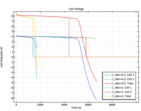
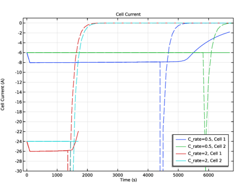
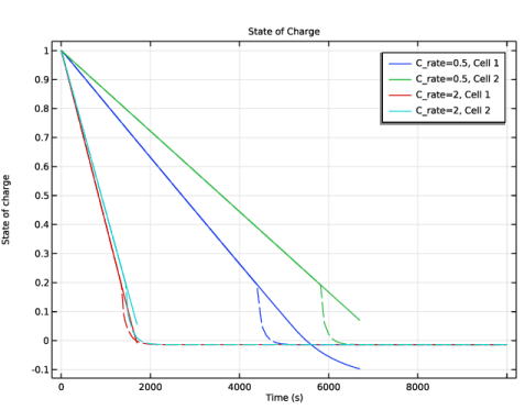
|
1
|
|
2
|
|
3
|
Click Add.
|
|
4
|
|
5
|
Click Add.
|
|
6
|
|
7
|
Click Add.
|
|
8
|
Click
 Study. Study. |
|
9
|
|
10
|
Click
 Done. Done. |
|
1
|
|
2
|
|
3
|
Click
 Load from File. Load from File. |
|
4
|
Browse to the model’s Application Libraries folder and double-click the file overdischarge_protection_parameters.txt.
|
|
1
|
|
2
|
|
1
|
|
2
|
|
3
|
|
4
|
|
5
|
Click
 Import. Import. |
|
6
|
Locate the Interpolation and Extrapolation section. From the Extrapolation list, choose Nearest function.
|
|
7
|
|
8
|
In the Function table, enter the following settings:
|
|
1
|
|
2
|
|
3
|
|
4
|
|
5
|
|
1
|
In the Model Builder window, under Component 1 (comp1) > Lumped Battery (lb) click Cell Equilibrium Potential 1.
|
|
2
|
|
3
|
|
4
|
|
1
|
|
2
|
|
3
|
|
4
|
|
5
|
Locate the Concentration Overpotential section. Select the Include concentration overpotential checkbox.
|
|
6
|
|
1
|
|
2
|
|
3
|
|
1
|
|
2
|
|
3
|
|
4
|
|
5
|
|
1
|
In the Model Builder window, under Component 1 (comp1) > Lumped Battery 2 (lb2) click Cell Equilibrium Potential 1.
|
|
2
|
|
3
|
|
4
|
|
1
|
|
2
|
|
3
|
|
4
|
|
5
|
Locate the Concentration Overpotential section. Select the Include concentration overpotential checkbox.
|
|
6
|
|
1
|
|
2
|
|
4
|
|
1
|
|
2
|
|
3
|
Locate the Node Connections section. In the table, enter the following settings:
|
|
4
|
|
1
|
|
2
|
|
3
|
Locate the Node Connections section. In the table, enter the following settings:
|
|
4
|
Locate the External Device section. From the V list, choose Electric potential on circuit (lb2/vl1).
|
|
1
|
|
2
|
|
4
|
|
1
|
|
2
|
|
1
|
|
2
|
|
3
|
|
1
|
|
2
|
|
3
|
|
4
|
|
5
|
|
6
|
Click
 Add. Add. |
|
1
|
|
2
|
|
3
|
In the Model Builder window, expand the Study 1: Without Shunts > Solver Configurations > Solution 1 (sol1) > Time-Dependent Solver 1 node.
|
|
4
|
Right-click Study 1: Without Shunts > Solver Configurations > Solution 1 (sol1) > Time-Dependent Solver 1 and choose Stop Condition.
|
|
5
|
|
6
|
Click
 Add. Add. |
|
8
|
|
1
|
|
2
|
|
3
|
|
4
|
|
5
|
Locate the Plot Settings section.
|
|
6
|
|
7
|
|
1
|
|
2
|
|
3
|
|
4
|
Click Add Expression in the upper-right corner of the y-Axis Data section. From the menu, choose Component 1 (comp1) > Lumped Battery > lb.E_cell - Cell potential - V.
|
|
5
|
Locate the y-Axis Data section. In the table, enter the following settings:
|
|
6
|
Click Add Expression in the upper-right corner of the y-Axis Data section. From the menu, choose Component 1 (comp1) > Lumped Battery 2 > lb2.E_cell - Cell potential - V.
|
|
7
|
Locate the y-Axis Data section. In the table, enter the following settings:
|
|
8
|
Click Add Expression in the upper-right corner of the y-Axis Data section. From the menu, choose Component 1 (comp1) > Electrical Circuit > Measurements > cir.vm1.v - Voltage across Volt meter vm1 - V.
|
|
9
|
Locate the y-Axis Data section. In the table, enter the following settings:
|
|
10
|
|
11
|
|
12
|
|
1
|
|
2
|
|
3
|
|
4
|
|
5
|
|
6
|
|
1
|
|
2
|
|
3
|
Click
 Clear Table. Clear Table. |
|
4
|
Click Replace Expression in the upper-right corner of the y-Axis Data section. From the menu, choose Component 1 (comp1) > Lumped Battery > lb.I_cell - Cell current - A.
|
|
5
|
Locate the y-Axis Data section. In the table, enter the following settings:
|
|
6
|
Click Add Expression in the upper-right corner of the y-Axis Data section. From the menu, choose Component 1 (comp1) > Lumped Battery 2 > lb2.I_cell - Cell current - A.
|
|
7
|
Locate the y-Axis Data section. In the table, enter the following settings:
|
|
8
|
|
1
|
|
2
|
|
3
|
|
4
|
|
5
|
Locate the Plot Settings section.
|
|
6
|
|
1
|
|
2
|
|
3
|
|
4
|
Click Add Expression in the upper-right corner of the y-Axis Data section. From the menu, choose Component 1 (comp1) > Lumped Battery > lb.SOC_cell - Cell state of charge - 1.
|
|
5
|
Locate the y-Axis Data section. In the table, enter the following settings:
|
|
6
|
Click Add Expression in the upper-right corner of the y-Axis Data section. From the menu, choose Component 1 (comp1) > Lumped Battery 2 > lb2.SOC_cell - Cell state of charge - 1.
|
|
7
|
Locate the y-Axis Data section. In the table, enter the following settings:
|
|
8
|
|
9
|
|
1
|
|
2
|
Go to the Add Physics window.
|
|
3
|
|
4
|
Click the Add to Component 1 button in the window toolbar.
|
|
5
|
|
1
|
|
2
|
|
1
|
|
2
|
|
1
|
|
2
|
|
3
|
|
4
|
Locate the Reinitialization section. In the table, enter the following settings:
|
|
1
|
|
2
|
|
3
|
|
4
|
Locate the Reinitialization section. In the table, enter the following settings:
|
|
1
|
|
2
|
|
3
|
|
4
|
Locate the Node Connections section. In the table, enter the following settings:
|
|
1
|
|
2
|
|
3
|
Locate the Node Connections section. In the table, enter the following settings:
|
|
4
|
|
1
|
|
2
|
Go to the Add Study window.
|
|
3
|
|
4
|
Click the Add Study button in the window toolbar.
|
|
5
|
|
1
|
|
2
|
|
3
|
|
4
|
|
5
|
Click
 Add. Add. |
|
7
|
|
8
|
|
9
|
Clear the Generate default plots checkbox.
|
|
10
|
|
1
|
|
2
|
|
1
|
In the Model Builder window, under Results > Cell Voltage right-click Global 1 and choose Duplicate.
|
|
2
|
|
3
|
|
4
|
Locate the Coloring and Style section. Find the Line style subsection. From the Line list, choose Dashed.
|
|
5
|
|
6
|
|
7
|
|
1
|
In the Model Builder window, under Results > Cell Current right-click Global 1 and choose Duplicate.
|
|
2
|
|
3
|
|
4
|
Locate the Coloring and Style section. Find the Line style subsection. From the Line list, choose Dashed.
|
|
5
|
|
1
|
|
2
|
|
3
|
|
1
|
|
2
|
|
3
|
|
4
|
Locate the Coloring and Style section. Find the Line style subsection. From the Line list, choose Dashed.
|
|
5
|
|
6
|
|
7
|


