PDF

Minimizing the Charging Time of a Lithium-Ion Battery
Introduction
Optimizing a fast-charging curve for a battery is a multiple-objective problem. At the same time as one strives to minimize the total charging time, the applied high charge rates must not result in excessive aging of the battery. In a typical fast charge cycle for a lithium-ion battery, the initially high charging current is continuously lowered in order not to induce lithium plating or accelerated solid electrolyte interphase (SEI) formation.
This model extends the Lithium-Ion Battery Base Model in 1D with an optimization study, with the objective to minimize the required charging time for charging the battery from 0 to 90% state of charge (SOC). This is achieved by fitting the shape of the charging profile using a control function, subject to a constraint for the maximum allowed degradation during the charge cycle.
Model Definition
Charge Curve Definition and the Control Function
The C rate of a battery is proportional to the battery current, where a C rate of 1 equals the current required to fully charge, or discharge, the battery in 1 h. A total current condition is used as boundary condition for the battery model, with the applied current defined as
(1)
Here, Qcell is the battery capacity as defined by the Lithium-Ion Battery interface.
The charging function C is defined using a Control Function, based on a five-segment piecewise Bernstein polynomial, resulting in seven control variables (fitting parameters). The argument for the control function, ranging between 0 and 1, represents a dimensionless time , scaled so that the value 0 represents the time at the beginning of the charge cycle and 1 the final time when the battery has reached the target SOC of 90%. By this definition, the area of the control function equals the average C-rate over the whole charge cycle.
(2)
and the time scale, tscale, can be computed as
(3)
A stop expression is enabled in optimization study in order to stop the time-dependent solver when the battery has reached 90% SOC (at t = tscale).
The optimization solver is set to maximize the value of the variable Cavg.
Constraining the parasitic reactions
The amount of degradation during the charging cycle is computed using a generalized volumetric Butler–Volmer expression in the negative graphite electrode of the following form.
(4)
where the overpotential η is defined as
(5)
The volumetric current is defined to be zero for positive (anodic) overpotentials by the expression
(6)
The above parasitic aging expression was chosen for tutorial purposes, but could represent, for instance, irreversible SEI formation with an onset potential of 25 mV, or lithium plating (with an added safety margin of 25 mV).
Integrating the volumetric current density in the negative electrode over the course of the whole simulation gives a measure of the total amount of capacity lost due to the parasitic reaction
(7)
During optimization, charging profiles that result in a degradation larger than 10% over 1000 cycles are prohibited by defining a constraint variable as
(8)
The above variable is used as a constraint expression optimization solver, with an upper bound of 1.
Results and Discussion
Figure 1 compares the initial loading cycle with the optimized one.
Figure 1: The optimized charge profile is plotted together with the electroplating current.
The optimization reduces the charging time by a factor of 2 relative to the initial charging profile, but this comes at the cost of a nonzero electroplating current. The relationship between these two objectives is plotted in Figure 2, where the charging profile has been optimized for different values of the maximum number of cycles. The figure shows that it is possible to achieve a tenfold improvement in longevity for the battery at the cost of a 20% increase in the charging time.
Figure 2: The maximum number of cycles is plotted as a function of the charging time.
Application Library path: Battery_Design_Module/Lithium-Ion_Batteries,_Performance/lib_charge_rate_optimization
Modeling Instructions
This example starts from an existing model from the Battery Design Module Application Library.
Application Libraries
1
From the File menu, choose Application Libraries.
2
In the Application Libraries window, select Battery Design Module > Lithium-Ion Batteries, Performance > lib_base_model_1d in the tree.
3
Global Definitions
Parameters 1
1
In the Model Builder window, under Global Definitions click Parameters 1.
2
In the Settings window for Parameters, locate the Parameters section.
3
Optimization Parameters
1
In the Home toolbar, click  Parameters and choose Add > Parameters.
2
In the Settings window for Parameters, type Optimization Parameters in the Label text field.
3
Locate the Parameters section. In the table, enter the following settings:
Use a Control Function to optimize the nondimensional charging rate.
Definitions (comp1)
Control Function 1 (cfunc1)
1
In the Definitions toolbar, click  Control Variables and choose Control Function.
2
In the Settings window for Control Function, locate the Output section.
3
In the fmax text field, type 4.
4
In the c0 text field, type 1.
5
Locate the Control Variable Discretization section. From the Control type list, choose Piecewise Bernstein polynomial.
6
Locate the Output section. In the c0 text field, type cfunc0.
7
Locate the Units section. Click  Select Input Quantity.
8
In the Physical Quantity dialog, select General > Dimensionless (1) in the tree.
9
Variables 2 - Negative Electrode
1
In the Model Builder window, under Component 1 (comp1) right-click Definitions and choose Variables.
2
In the Settings window for Variables, type Variables 2 - Negative Electrode in the Label text field.
3
Locate the Geometric Entity Selection section. From the Geometric entity level list, choose Domain.
4
From the Selection list, choose Negative Electrode.
5
Locate the Variables section. In the table, enter the following settings:
Domain Probe 1 (dom1)
1
In the Definitions toolbar, click  Probes and choose Domain Probe.
2
In the Settings window for Domain Probe, type total_aging_current in the Variable name text field.
3
Locate the Probe Type section. From the Type list, choose Integral.
4
Locate the Source Selection section. From the Selection list, choose Negative Electrode.
5
Click Replace Expression in the upper-right corner of the Expression section. From the menu, choose Component 1 (comp1) > Definitions > Variables > i_aging - Parasitic aging current density to use in constraint variable - A/m³.
6
Locate the Expression section. In the Expression text field, type -i_aging*A_cell.
Lithium-Ion Battery (liion)
Electrode Current 1
1
In the Model Builder window, expand the Study 1 node.
2
Right-click Component 1 (comp1) > Lithium-Ion Battery (liion) and choose Electrode Phase > Electrode Current.
3
4
In the Settings window for Electrode Current, locate the Electrode Current section.
5
From the list, choose C-rate multiple.
6
In the Crate text field, type cfunc1(t*avg_C_rate/t_1C).
Using cfunc1(t*avg_C_rate/t_1C) instead of cfunc1(t) ensures that the entire range of the Control Function is utilized.
Load Cycle 1
In the Model Builder window, right-click Load Cycle 1 and choose Delete.
Particle Intercalation 1
1
In the Model Builder window, expand the Component 1 (comp1) > Lithium-Ion Battery (liion) > Porous Electrode - Negative node, then click Particle Intercalation 1.
2
In the Settings window for Particle Intercalation, click to expand the Particle Discretization section.
3
Select the Fast assembly in particle dimension checkbox to reduce the computational time.
Particle Intercalation 1
1
In the Model Builder window, expand the Component 1 (comp1) > Lithium-Ion Battery (liion) > Porous Electrode - Positive node, then click Particle Intercalation 1.
2
In the Settings window for Particle Intercalation, locate the Particle Discretization section.
3
Select the Fast assembly in particle dimension checkbox.
Component 1 (comp1)
Add an ODE to compute the parasitic aging charge as the integral of the parasitic aging current.
Add Physics
1
In the Home toolbar, click  Windows and choose Add Physics.
2
Go to the Add Physics window.
3
In the tree, select Mathematics > ODE and DAE Interfaces > Global ODEs and DAEs (ge).
4
Click the Add to Component 1 button in the window toolbar.
5
In the Home toolbar, click  Add Physics to close the Add Physics window.
Global ODEs and DAEs (ge)
Global Equations 1 (ODE1)
1
In the Settings window for Global Equations, locate the Global Equations section.
2
3
Locate the Units section. Click  Define Dependent Variable Unit.
4
In the Dependent variable quantity table, enter the following settings:
5
Click  Select Source Term Quantity.
6
In the Physical Quantity dialog, select General > Current (A) in the tree.
7
Definitions (comp1)
Variables 1 - Global
1
In the Model Builder window, under Component 1 (comp1) > Definitions click Variables 1.
2
In the Settings window for Variables, type Variables 1 - Global in the Label text field.
3
Locate the Variables section. In the table, enter the following settings:
This corresponds to allowing a degradation of 10% after 1000 cycles.
Study 1
Step 1: Current Distribution Initialization
1
In the Model Builder window, expand the Study 1 node, then click Step 1: Current Distribution Initialization.
2
In the Settings window for Current Distribution Initialization, locate the Physics and Variables Selection section.
3
In the Solve for column of the table, under Component 1 (comp1), clear the checkbox for Global ODEs and DAEs (ge).
Step 2: Time Dependent
1
In the Model Builder window, click Step 2: Time Dependent.
2
In the Settings window for Time Dependent, locate the Study Settings section.
3
In the Output times text field, type range(0,0.1/cfunc0,0.9/cfunc0).
4
Click to expand the Results While Solving section. From the Probes list, choose None.
5
In the Model Builder window, click Study 1.
6
In the Settings window for Study, type Study 1: Initial in the Label text field.
7
In the Study toolbar, click  Compute.
Results
1D Plot Group 7
1
In the Model Builder window, expand the Results > 1D Plot Group 7 node.
2
Right-click 1D Plot Group 7 and choose Delete.
Study 1: Initial
1
In the Model Builder window, click Study 1: Initial.
2
In the Settings window for Study, locate the Study Settings section.
3
Clear the Generate default plots checkbox.
Parametric Sweep
1
In the Study toolbar, click  Parametric Sweep.
2
In the Settings window for Parametric Sweep, locate the Study Settings section.
3
4
5
Locate the Output While Solving section. From the Probes list, choose None.
6
In the Study toolbar, click  Compute.
Add Study
1
In the Home toolbar, click  Windows and choose Add Study.
2
Go to the Add Study window.
3
Find the Studies subsection. In the Select Study tree, select Empty Study.
4
Click the Add Study button in the window toolbar.
5
In the Home toolbar, click  Add Study to close the Add Study window.
Study 1: Initial
Step 1: Current Distribution Initialization, Step 2: Time Dependent
1
In the Model Builder window, under Study 1: Initial, Ctrl-click to select Step 1: Current Distribution Initialization and Step 2: Time Dependent.
2
Study 2
In the Model Builder window, right-click Study 2 and choose Paste Multiple Items.
General Optimization
1
In the Study toolbar, click  Optimization and choose General Optimization.
2
In the Settings window for General Optimization, locate the Optimization Solver section.
3
From the Method list, choose GCMMA.
4
From the Study step list, choose Time Dependent.
5
Click Add Expression in the upper-right corner of the Objective Function section. From the menu, choose Component 1 (comp1) > Definitions > Variables > comp1.avg_C_rate - Average C rate (to be maximized) - 1.
6
Locate the Objective Function section. From the Type list, choose Maximization.
7
Select the Condition-based final time checkbox.
8
In the Stop expression text field, type t_1C-t*comp1.avg_C_rate, so that the total charge becomes fixed.
9
Click Add Expression in the upper-right corner of the Constraints section. From the menu, choose Component 1 (comp1) > Definitions > Variables > comp1.constr - Constraint - 1.
10
Locate the Constraints section. In the table, enter the following settings:
11
Click to expand the Output section. From the Probes list, choose None.
Step 2: Time Dependent
1
In the Model Builder window, click Step 2: Time Dependent.
2
In the Settings window for Time Dependent, locate the Study Settings section.
3
In the Output times text field, type range(0,0.01[h],3*t_1C).
4
In the Model Builder window, click Study 2.
5
In the Settings window for Study, type Study 2: Optimization in the Label text field.
6
Locate the Study Settings section. Clear the Generate default plots checkbox.
7
In the Study toolbar, click  Get Initial Value, so that a plot can be setup to be shown while solving.
Results
Control Function
1
In the Results toolbar, click  1D Plot Group.
2
In the Settings window for 1D Plot Group, locate the Data section.
3
From the Dataset list, choose Study 2: Optimization/Solution 8 (sol8).
4
In the Label text field, type Control Function.
5
Click to expand the Title section. From the Title type list, choose Manual.
6
In the Title text area, type constr = eval(constr).
Global 1
1
Right-click Control Function and choose Global.
2
In the Settings window for Global, locate the y-Axis Data section.
3
4
Locate the x-Axis Data section. From the Parameter list, choose Expression.
5
In the Expression text field, type t.
6
From the Unit list, choose min.
Global 2
1
Right-click Global 1 and choose Duplicate.
2
In the Settings window for Global, click Replace Expression in the upper-right corner of the y-Axis Data section. From the menu, choose Component 1 (comp1) > Definitions > total_aging_current - Domain Probe 1 - A.
3
Locate the y-Axis Data section. In the table, enter the following settings:
Global 3
1
In the Model Builder window, under Results > Control Function right-click Global 1 and choose Duplicate.
2
In the Settings window for Global, locate the Data section.
3
From the Dataset list, choose Study 1: Initial/Solution 1 (sol1).
4
In the Control Function toolbar, click  Plot.
5
Locate the y-Axis Data section. In the table, enter the following settings:
6
Click to expand the Coloring and Style section. From the Color list, choose Cycle (reset).
7
Find the Line style subsection. From the Line list, choose Dashed.
Global 4
1
In the Model Builder window, under Results > Control Function right-click Global 2 and choose Duplicate.
2
In the Settings window for Global, locate the Data section.
3
From the Dataset list, choose Study 1: Initial/Solution 1 (sol1).
4
Locate the y-Axis Data section. In the table, enter the following settings:
5
Locate the Coloring and Style section. Find the Line style subsection. From the Line list, choose Dashed.
Control Function
1
In the Model Builder window, click Control Function.
2
In the Settings window for 1D Plot Group, locate the Plot Settings section.
3
Select the Two y-axes checkbox.
4
In the table, select the Plot on secondary y-axis checkboxes for Global 2 and Global 4.
5
Select the y-axis label checkbox. In the associated text field, type C rate (1).
6
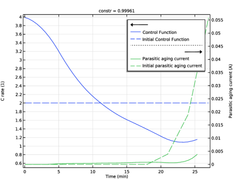
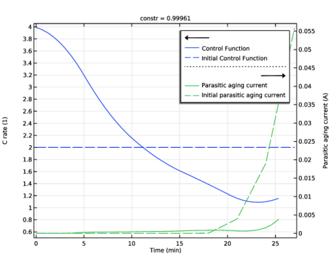
Select the Secondary y-axis label checkbox. In the associated text field, type Parasitic aging current (A).
Study 2: Optimization
General Optimization
1
In the Model Builder window, under Study 2: Optimization click General Optimization.
2
In the Settings window for General Optimization, locate the Output section.
3
Select the Plot checkbox.
4
Solver Configurations
In the Model Builder window, expand the Study 2: Optimization > Solver Configurations node.
Solution 8 (sol8)
1
In the Model Builder window, expand the Study 2: Optimization > Solver Configurations > Solution 8 (sol8) > Optimization Solver 1 > Time-Dependent Solver 1 node, then click Advanced.
2
In the Settings window for Advanced, click to expand the Assembly Settings section.
3
Clear the Reuse sparsity pattern checkbox to avoid messages in the log for every reassembly of the sparsity pattern.
Use a Parametric Sweep to investigate the relative cost of degradation versus charging rate for optimal charging profiles.
Parametric Sweep
1
In the Study toolbar, click  Parametric Sweep.
2
In the Settings window for Parametric Sweep, locate the Study Settings section.
3
4
5
Locate the Output While Solving section. From the Probes list, choose None.
6
Click to expand the Advanced Settings section. Select the Reuse solution from previous step checkbox to reduce the computational time.
7
In the Study toolbar, click  Compute.
Results
Control Function
1
In the Settings window for 1D Plot Group, locate the Axis section.
2
Select the Manual axis limits checkbox.
3
In the y minimum text field, type 0.5.
4
In the Control Function toolbar, click  Plot.
Pareto-Optimal Front
1
In the Home toolbar, click  Add Plot Group and choose 1D Plot Group.
2
In the Settings window for 1D Plot Group, type Pareto-Optimal Front in the Label text field.
3
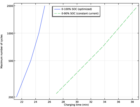
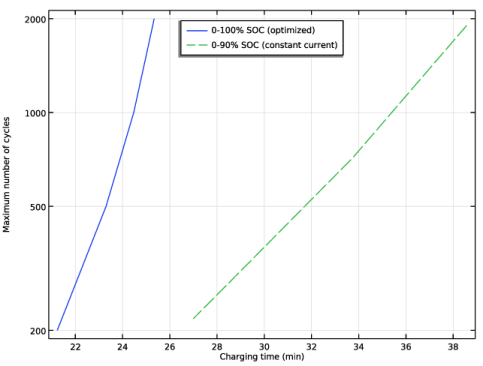
Locate the Data section. From the Dataset list, choose Study 2: Optimization/Parametric Solutions 2 (sol10).
4
From the Time selection list, choose Last.
5
Locate the Title section. From the Title type list, choose None.
6
Locate the Plot Settings section.
7
Select the y-axis label checkbox. In the associated text field, type Maximum number of cycles.
8
Locate the Axis section. Select the y-axis log scale checkbox.
9
Locate the Legend section. From the Position list, choose Upper middle.
Global 1
1
Right-click Pareto-Optimal Front and choose Global.
2
In the Settings window for Global, locate the y-Axis Data section.
3
4
Locate the x-Axis Data section. From the Axis source data list, choose Outer solutions.
5
From the Parameter list, choose Expression.
6
In the Expression text field, type t_1C/cfunc1.avg.
7
From the Unit list, choose min.
8
Select the Description checkbox. In the associated text field, type Charging time.
9
Click to expand the Legends section. Find the Include subsection. Clear the Solution checkbox.
Global 2
1
Right-click Global 1 and choose Duplicate.
2
In the Settings window for Global, locate the Data section.
3
From the Dataset list, choose Study 1: Initial/Parametric Solutions 1 (sol3).
4
From the Time selection list, choose Last.
5
Locate the y-Axis Data section. In the table, enter the following settings:
6
Locate the x-Axis Data section. From the Axis source data list, choose All solutions.
7
Locate the Coloring and Style section. Find the Line style subsection. From the Line list, choose Dashed.
8
Locate the x-Axis Data section. In the Expression text field, type t.
9
In the Pareto-Optimal Front toolbar, click  Plot.