PDF

Lithium Plating and Stripping
Introduction
Lithium plating on the negative electrode in preference to lithium intercalation is known to reduce capacity and to be a safety concern for lithium-ion batteries. Harsh charge conditions such as high currents (fast charging) and/or low temperatures can lead to lithium plating. The plated lithium is partially reversible in a process called stripping during battery discharge.
This example shows how to model the lithium plating/stripping reaction in the negative graphite electrode in a lithium-ion battery. The resulting capacity loss is predicted for different C-rates and temperatures. The example demonstrates how the Porous Electrode node can incorporate the electrochemical plating/stripping reaction.
Model Definition
general
The model is set up in 1D for a graphite/NMC battery cell using a 1.0 M LiPF6 in EC:EMC (3:7 by weight) electrolyte. Properties for these materials are taken from the Battery material library.
The model consists of the following three domains:
Negative porous electrode: Graphite (MCMB LixC6) active material (~112 μm).
Separator (30 μm).
The Arrhenius equation is used to model the temperature variation of the intercalation exchange current densities. In addition, temperature-dependent electrolyte properties are defined automatically by adding the electrolyte from the material library.
The Lithium-Ion Battery interface is used, accounting for:
More information on the general description can be found in the 1D Isothermal Lithium-Ion Battery example. The lithium plating/stripping formulations are based on the investigations in Ref. 1Ref. 3 and the details are presented below.
Lithium plating/stripping Reaction
The lithium plating/stripping is defined as an additional reaction to the main graphite-lithium intercalation reaction on the negative electrode. This is done using an additional Porous Electrode Reaction in the Porous Electrode node for the negative electrode.
The plating is considered to be a pure electrochemical reaction:
The reverse reaction, stripping, is considered to only partially dissolve the plated lithium electrochemically. The remaining plated lithium is regarded to be irreversibly lost (a loss in lithium inventory) and is often referred to as “dead lithium” (Ref. 1). The stoichiometric coefficient of the dead lithium fraction, YLi, dead, is set to 0.1 in this example, can be incorporated into the stripping reaction expression in the following way:
The electrochemical reaction current, iLi, is defined by concentration-dependent Butler–Volmer kinetics:
(1)
where the pre-exponential factor for the anodic term Fa is defined as:
(2)
In the expressions above
i0,ref is the reference exchange current density defined at 1 M lithium ion concentration.
cl is the lithium ion concentration in the electrolyte.
cl,ref is the reference lithium ion concentration, equal to 1 M.
cLi(s),cov is the concentration of a monolayer fully covered with plated lithium on the negative active material. The monolayer thickness is set to 0.1 nm.
  cLi(s) is the plated lithium concentration.
ηLi is the lithium plating/stripping overpotential in which the equilibrium potential, Eeq,Li, is 0 V versus lithium:
(3)
The plated and dead lithium concentrations, cLi(s) and cLi, Dead, are computed using the in-built Dissolving–Depositing Species feature in the main Porous Electrode node. The dissolving–deposited concentrations are computed by integrating the reaction source/sink terms using the following two equations:
(4)
(5)
where av is the specific surface area (m2/m3) of the active material particles.
The stoichiometric coefficients, νLi(s) and νLi, Dead, follow the reaction expression above and are set as follows:
For plating, iplate < 0:
(6)
(7)
For stripping, iplate > 0:
(8)
(9)
Charge–Discharge cycle
To evaluate the plating/stripping reaction, a full charge-discharge cycle is simulated. The upper and lower cutoff voltages are set to 4.2 V and 2.7 V, respectively. The cycle consists of a constant current charge period up to the upper cutoff voltage followed by a constant voltage charge period at the upper cutoff voltage and a constant current discharge period to the lower cutoff voltage. The battery is set to be completely discharged initially.
Results and Discussion
To investigate the impact of current, the charge-discharge cycle is simulated for three different constant current rates (C-rates) at 298 K. The influence of temperature is studied by simulating the cycle for 1C current at three different temperatures.
The cell voltages as functions of SOC are displayed in Figure 1 and Figure 2 for the C-rate and temperature studies, respectively. Large variations with cycling conditions are shown.
Figure 1: Cell voltage versus SOC for 1C, 3C, and 5C charge-discharge cycles at 298 K.
Figure 2: Cell voltage versus SOC at 298 K, 283 K, and 268 K for 1C charge-discharge cycle.
The susceptibility to plating can be seen in the electrode potential at the negative electrode. A potential equal to or lower than 0 V is indicative of lithium plating. In Figure 3 and Figure 4, the electrode potential at the electrode-separator and current collector-electrode boundaries are shown during charge. The former boundary is most susceptible to lithium plating in all results. The lowest cell temperature case has a potential below 0 V for a long period during charge.
Figure 3: Negative electrode potential at the electrode–separator and current collector–electrode boundaries for 1C, 3C, and 5C charge-discharge cycles at 298 K.
Figure 4: Negative electrode potential at the electrode–separator and current collector–electrode boundaries at 298 K, 283 K, and 268 K for 1C charge-discharge cycle.
The total lithium film thickness, that is, plated and dead lithium, at the electrode–separator interface is displayed in Figure 5 and Figure 6 over the cycle. Increased C-rate increases the plating to some extent. Lowered temperature increases the plating to the greatest extent. Most of the plating is reversible during the cycle. The irreversible part is due to the formation of dead lithium and reduces the lithium inventory.
Figure 5: Total lithium film thickness variation at the electrode-separator boundary for 1C, 3C, and 5C at 298 K.
Figure 6: Total lithium film thickness variation at the electrode–separator boundary for 298 K, 283 K, and 268 K at 1C constant current rate.
In the two last figures (Figure 7 and Figure 8), the amount of dead lithium in terms of lithium inventory loss in the cell during cycling is shown. The loss is substantial at the lowest temperature, in all other cases most of the lithium is reversible.
Figure 7: Lithium inventory loss for 1C, 3C, and 5C cycles at 298 K.
Figure 8: Lithium inventory loss for 298 K, 283 K, and 268 K cycles at 1C constant current rate.
References
1. S.E.J. O’Kane, I.D. Campbell, M.W.J. Marzook, G.J. Offer, and M. Marinescu, “Physical Origin of the Differential Voltage Minimum Associated with Lithium Plating in Li-Ion Batteries,” J. Elec. Soc., vol. 167, pp. 090540, 2020.
2. X.-G. Yang, S. Ge, T. Liu, Y. Leng, and C.-Y. Wang, “A look into the voltage plateau signal for detection and quantification of lithium plating in lithium-ion cells,” J. Power Sources, vol. 395, pp. 251–261, 2018.
3. S.E.J. O’Kane, W. Ai, G. Madabattula, D. Alonso-Alvarez, R. Timms, V. Sulzer, J.S. Edge, B. Wu, G.J. Offer, and M. Marinescu, “Lithium-ion battery degradation: how to model it,” Phys. Chem. Chem. Phys., vol. 24, pp. 7909–7922, 2022.
Application Library path: Battery_Design_Module/Lithium-Ion_Batteries,_Aging_and_Abuse/li_plating
Modeling Instructions
From the File menu, choose New.
New
In the New window, click  Model Wizard.
Model Wizard
1
In the Model Wizard window, click  1D.
2
In the Select Physics tree, select Electrochemistry > Batteries > Lithium-Ion Battery (liion).
3
Click Add.
4
Click  Study.
5
In the Select Study tree, select Preset Studies for Selected Physics Interfaces > Time Dependent with Initialization.
6
Global Definitions
Model Parameters
1
In the Model Builder window, under Global Definitions click Parameters 1.
2
In the Settings window for Parameters, type Model Parameters in the Label text field.
Load the parameters from a text file.
3
Locate the Parameters section. Click  Load from File.
4
Add Material
1
In the Materials toolbar, click  Add Material to open the Add Material window.
Add some data for the electrolyte and the electrodes from the material library.
2
Go to the Add Material window.
3
In the tree, select Battery > Electrolytes > LiPF6 in 3:7 EC:EMC (Liquid, Li-ion Battery).
4
Right-click and choose Add to Component 1 (comp1).
5
In the tree, select Battery > Electrodes > Graphite, LixC6 MCMB (Negative, Li-ion Battery).
6
Right-click and choose Add to Component 1 (comp1).
7
In the tree, select Battery > Electrodes > NMC 811, LiNi0.8Mn0.1Co0.1O2 (Positive, Li-ion Battery).
8
Right-click and choose Add to Component 1 (comp1).
9
In the Materials toolbar, click  Add Material to close the Add Material window.
Geometry 1
Draw the model geometry by defining the individual thicknesses of the negative electrode, the separator, and the positive electrode.
Interval 1 (i1)
1
In the Model Builder window, under Component 1 (comp1) right-click Geometry 1 and choose Interval.
2
In the Settings window for Interval, locate the Interval section.
3
From the Specify list, choose Interval lengths.
4
5
Click  Build Selected.
Materials
LiPF6 in 3:7 EC:EMC (Liquid, Li-ion Battery) (mat1)
Now assign the previously added materials to the different domains of the geometry. Create selections at the same time to facilitate choosing the same domains later on.
1
In the Model Builder window, under Component 1 (comp1) > Materials click LiPF6 in 3:7 EC:EMC (Liquid, Li-ion Battery) (mat1).
2
3
In the Settings window for Material, locate the Geometric Entity Selection section.
4
Click  Create Selection.
5
In the Create Selection dialog, type Separator in the Selection name text field.
6
Graphite, LixC6 MCMB (Negative, Li-ion Battery) (mat2)
1
In the Model Builder window, click Graphite, LixC6 MCMB (Negative, Li-ion Battery) (mat2).
2
In the Settings window for Material, locate the Geometric Entity Selection section.
3
Click  Clear Selection.
4
5
Click  Create Selection.
6
In the Create Selection dialog, type Negative Electrode in the Selection name text field.
7
NMC 811, LiNi0.8Mn0.1Co0.1O2 (Positive, Li-ion Battery) (mat3)
1
In the Model Builder window, click NMC 811, LiNi0.8Mn0.1Co0.1O2 (Positive, Li-ion Battery) (mat3).
2
3
In the Settings window for Material, locate the Geometric Entity Selection section.
4
Click  Create Selection.
5
In the Create Selection dialog, type Positive Electrode in the Selection name text field.
6
Definitions
Add some variables for the electrodes.
Variables Positive Electrode
1
In the Model Builder window, under Component 1 (comp1) right-click Definitions and choose Variables.
2
In the Settings window for Variables, type Variables Positive Electrode in the Label text field.
3
Locate the Geometric Entity Selection section. From the Geometric entity level list, choose Domain.
4
From the Selection list, choose Positive Electrode.
5
Locate the Variables section. In the table, enter the following settings:
Variables Negative Electrode
1
Right-click Variables Positive Electrode and choose Duplicate.
2
In the Settings window for Variables, type Variables Negative Electrode in the Label text field.
3
Locate the Geometric Entity Selection section. From the Selection list, choose Negative Electrode.
4
Locate the Variables section. In the table, enter the following settings:
Integration - Negative
1
In the Definitions toolbar, click  Nonlocal Couplings and choose Integration.
2
In the Settings window for Integration, type Integration - Negative in the Label text field.
3
Locate the Source Selection section. From the Selection list, choose Negative Electrode.
4
In the Operator name text field, type negative.
Lithium-Ion Battery (liion)
Now start defining the physics. Use the SOC and Initial Charge Distribution node to calculate the initial charge distribution in the cell.
1
In the Model Builder window, under Component 1 (comp1) click Lithium-Ion Battery (liion).
2
In the Settings window for Lithium-Ion Battery, locate the Cross-Sectional Area section.
3
In the Ac text field, type A_cell.
4
Locate the Cell Settings section. Select the Define cell state of charge (SOC) and initial charge inventory checkbox.
SOC and Initial Charge Distribution 1
1
In the Model Builder window, under Component 1 (comp1) > Lithium-Ion Battery (liion) click SOC and Initial Charge Distribution 1.
2
In the Settings window for SOC and Initial Charge Distribution, locate the State-of-Charge Definition section.
3
From the list, choose User defined. In the Ecell0%SOC text field, type Vlow.
4
In the Ecell100%SOC text field, type Vhigh.
5
Locate the Initial Cell Charge Distribution section. In the SOC0 text field, type SOCcell_init.
6
In the floss,neg text field, type Li_loss.
Negative Electrode Domain Selection 1
1
In the Model Builder window, click Negative Electrode Domain Selection 1.
2
In the Settings window for Negative Electrode Domain Selection, locate the Domain Selection section.
3
From the Selection list, choose Negative Electrode.
Positive Electrode Domain Selection 1
1
In the Model Builder window, click Positive Electrode Domain Selection 1.
2
In the Settings window for Positive Electrode Domain Selection, locate the Domain Selection section.
3
From the Selection list, choose Positive Electrode.
Separator 1
1
In the Model Builder window, under Component 1 (comp1) > Lithium-Ion Battery (liion) click Separator 1.
2
In the Settings window for Separator, locate the Porous Matrix Properties section.
3
In the εl text field, type epsl_sep.
Porous Electrode - Negative
1
In the Physics toolbar, click  Domains and choose Porous Electrode.
In the negative electrode, add lithium metal and dead lithium as dissolving-depositing species. Allow only volume changes due to lithium plating/stripping affect the electrolyte volume fraction.
2
In the Settings window for Porous Electrode, type Porous Electrode - Negative in the Label text field.
3
Locate the Domain Selection section. From the Selection list, choose Negative Electrode.
4
Locate the Electrolyte Properties section. From the Electrolyte material list, choose LiPF6 in 3:7 EC:EMC (Liquid, Li-ion Battery) (mat1).
5
Locate the Electrode Properties section. In the σs text field, type sigmas_neg.
6
Locate the Porous Matrix Properties section. In the εs text field, type epss_neg.
7
In the εl text field, type epsl_neg.
8
Locate the Effective Transport Parameter Correction section. From the Electric conductivity list, choose No correction.
9
Click to expand the Dissolving–Depositing Species section. Click  Add.
10
11
12
Clear the Add volume change to electrode volume fraction checkbox.
Particle Intercalation 1
1
In the Model Builder window, click Particle Intercalation 1.
2
In the Settings window for Particle Intercalation, locate the Particle Transport Properties section.
3
In the rp text field, type rp_neg.
Porous Electrode Reaction - Intercalation
1
In the Model Builder window, under Component 1 (comp1) > Lithium-Ion Battery (liion) > Porous Electrode - Negative click Porous Electrode Reaction 1.
2
In the Settings window for Porous Electrode Reaction, type Porous Electrode Reaction - Intercalation in the Label text field.
3
Locate the Electrode Kinetics section. In the i0,ref(T) text field, type Arreh*i0_ref_neg.
Porous Electrode Reaction - Lithium Plating and Stripping
1
In the Model Builder window, right-click Porous Electrode Reaction - Intercalation and choose Duplicate.
Define the lithium plating/stripping reaction in an additional porous electrode reaction node. A fraction, Ydead, will form dead lithium during stripping.
2
In the Settings window for Porous Electrode Reaction, type Porous Electrode Reaction - Lithium Plating and Stripping in the Label text field.
3
Locate the Equilibrium Potential section. From the Eeq list, choose User defined. Locate the Electrode Kinetics section. From the Kinetics expression type list, choose Concentration dependent kinetics.
4
In the i0 text field, type i0_ref_LiMetal*(cl/1[M])^0.5.
5
In the CR text field, type min(liion.c_pce1_LiMetal/(cLicov*liion.Av_pce1_per2),1).
6
Locate the Stoichiometric Coefficients section. In the νLiθ text field, type 0.
7
In the Stoichiometric coefficients for dissolving–depositing species: table, enter the following settings:
Porous Electrode - Positive
1
In the Physics toolbar, click  Domains and choose Porous Electrode.
2
In the Settings window for Porous Electrode, type Porous Electrode - Positive in the Label text field.
3
Locate the Domain Selection section. From the Selection list, choose Positive Electrode.
4
Locate the Electrolyte Properties section. From the Electrolyte material list, choose LiPF6 in 3:7 EC:EMC (Liquid, Li-ion Battery) (mat1).
5
Locate the Electrode Properties section. In the σs text field, type sigmas_pos.
6
Locate the Porous Matrix Properties section. In the εs text field, type epss_pos.
7
In the εl text field, type epsl_pos.
Particle Intercalation 1
1
In the Model Builder window, expand the Porous Electrode - Positive node, then click Particle Intercalation 1.
2
In the Settings window for Particle Intercalation, locate the Particle Transport Properties section.
3
In the rp text field, type rp_pos.
Porous Electrode Reaction 1
1
In the Model Builder window, click Porous Electrode Reaction 1.
2
In the Settings window for Porous Electrode Reaction, locate the Electrode Kinetics section.
3
In the i0,ref(T) text field, type Arreh*i0_ref_pos.
Electric Ground 1
1
In the Physics toolbar, click  Boundaries and choose Electric Ground.
2
3
In the Settings window for Electric Ground, locate the Boundary Selection section.
4
Click  Create Selection.
5
In the Create Selection dialog, type Negative CC in the Selection name text field.
6
Use the Charge-Discharge node to set up the load cycle (constant charge - constant voltage - constant discharge) between the cut-off limits.
Charge-Discharge Cycling 1
1
In the Physics toolbar, click  Boundaries and choose Charge-Discharge Cycling.
2
3
In the Settings window for Charge-Discharge Cycling, locate the Boundary Selection section.
4
Click  Create Selection.
5
In the Create Selection dialog, type Positive CC in the Selection name text field.
6
7
In the Settings window for Charge-Discharge Cycling, locate the Discharge Settings section.
8
From the list, choose C-rate multiple.
9
In the Crate,dch text field, type -C_rate.
10
In the Vmin text field, type Vlow.
11
Locate the Charge Settings section. From the list, choose C-rate multiple.
12
In the Crate,ch text field, type C_rate.
13
In the Vmax text field, type Vhigh.
14
Select the Include constant voltage charging checkbox.
15
In the Iupper text field, type I_taper.
16
Locate the Start Mode section. From the Start with list, choose Charge first.
Global Definitions
Default Model Inputs
1
In the Model Builder window, under Global Definitions click Default Model Inputs.
2
In the Settings window for Default Model Inputs, locate the Browse Model Inputs section.
3
In the tree, select General > Temperature (K) - minput.T.
4
Find the Expression for remaining selection subsection. In the Temperature text field, type T.
Mesh 1
1
In the Model Builder window, under Component 1 (comp1) click Mesh 1.
2
In the Settings window for Mesh, locate the Physics-Controlled Mesh section.
3
From the Element size list, choose Extremely fine.
4
Click  Build All.
Study - C-Rate
Use a parametric sweep to study the impact of the C-rate.
1
In the Model Builder window, click Study 1.
2
In the Settings window for Study, type Study - C-Rate in the Label text field.
Parametric Sweep
1
In the Study toolbar, click  Parametric Sweep.
2
In the Settings window for Parametric Sweep, locate the Study Settings section.
3
4
Step 2: Time Dependent
1
In the Model Builder window, click Step 2: Time Dependent.
2
In the Settings window for Time Dependent, locate the Study Settings section.
3
In the Output times text field, type range(0,100/C_rate,3600*6/C_rate).
4
In the Model Builder window, click Study - C-Rate.
5
In the Settings window for Study, locate the Study Settings section.
6
Clear the Generate default plots checkbox.
Solution 1 (sol1)
1
In the Study toolbar, click  Show Default Solver.
2
In the Model Builder window, expand the Solution 1 (sol1) node, then click Time-Dependent Solver 1.
3
In the Settings window for Time-Dependent Solver, locate the General section.
4
From the Times to store list, choose Steps taken by solver.
5
Right-click Study - C-Rate > Solver Configurations > Solution 1 (sol1) > Time-Dependent Solver 1 and choose Stop Condition.
Define a stop condition that terminates the simulation at the lower cut-off limit at discharge.
6
In the Settings window for Stop Condition, locate the Stop Expressions section.
7
8
9
Locate the Output at Stop section. Clear the Add information checkbox.
10
In the Study toolbar, click  Compute.
Results
Start creating the model figures.
Cell Voltage, C-rate
1
In the Results toolbar, click  1D Plot Group.
2
In the Settings window for 1D Plot Group, locate the Data section.
3
From the Dataset list, choose Study - C-Rate/Parametric Solutions 1 (sol3).
4
Click to expand the Title section. From the Title type list, choose None.
5
In the Label text field, type Cell Voltage, C-rate.
6
Locate the Plot Settings section.
7
Select the x-axis label checkbox. In the associated text field, type SOC (%).
8
Select the y-axis label checkbox. In the associated text field, type Cell voltage (V).
9
Locate the Legend section. Select the Show legends checkbox.
10
From the Position list, choose Lower right.
Global 1
1
Right-click Cell Voltage, C-rate and choose Global.
2
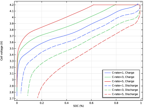
In the Settings window for Global, click Replace Expression in the upper-right corner of the y-Axis Data section. From the menu, choose Component 1 (comp1) > Lithium-Ion Battery > Charge-Discharge Cycling 1 > liion.cdc1.phis0 - Cell potential - V.
3
Click Replace Expression in the upper-right corner of the x-Axis Data section. From the menu, choose Component 1 (comp1) > Lithium-Ion Battery > liion.SOC_cell - Cell state of charge - 1.
4
Click to expand the Legends section. From the Legends list, choose Manual.
5
Filter 1
1
Right-click Global 1 and choose Filter.
2
In the Settings window for Filter, locate the Line Segment Selection section.
3
Clear the Decreasing x checkbox.
Global 2
1
In the Model Builder window, under Results > Cell Voltage, C-rate right-click Global 1 and choose Duplicate.
2
In the Settings window for Global, click to expand the Coloring and Style section.
3
Find the Line style subsection. From the Line list, choose Dashed.
4
From the Color list, choose Cycle (reset).
5
Locate the Legends section. From the Legends list, choose Manual.
6
Filter 1
1
In the Model Builder window, expand the Global 2 node, then click Filter 1.
2
In the Settings window for Filter, locate the Line Segment Selection section.
3
Clear the Increasing x checkbox.
4
Select the Decreasing x checkbox.
5
In the Cell Voltage, C-rate toolbar, click  Plot.
Lithium Plating Current, C-rate
1
In the Results toolbar, click  1D Plot Group.
2
In the Settings window for 1D Plot Group, type Lithium Plating Current, C-rate in the Label text field.
3
Locate the Data section. From the Dataset list, choose Study - C-Rate/Parametric Solutions 1 (sol3).
4
Locate the Title section. From the Title type list, choose None.
5
Locate the Plot Settings section.
6
Select the y-axis label checkbox. In the associated text field, type Plating/stripping current (A).
7
Locate the Legend section. Select the Show legends checkbox.
Global 1
1
Right-click Lithium Plating Current, C-rate and choose Global.
2
In the Settings window for Global, locate the y-Axis Data section.
3
4
Click to expand the Legends section. From the Legends list, choose Manual.
5
Global 2
1
Right-click Global 1 and choose Duplicate.
2
In the Settings window for Global, click to expand the Coloring and Style section.
3
Click Replace Expression in the upper-right corner of the y-Axis Data section. From the menu, choose Component 1 (comp1) > Lithium-Ion Battery > Charge-Discharge Cycling 1 > liion.cdc1.phis0 - Cell potential - V.
4
Locate the Coloring and Style section. Find the Line style subsection. From the Line list, choose Dashed.
5
From the Color list, choose Cycle (reset).
6
Locate the Legends section. In the table, enter the following settings:
Lithium Plating Current, C-rate
1
In the Model Builder window, click Lithium Plating Current, C-rate.
2
In the Settings window for 1D Plot Group, locate the Plot Settings section.
3
Select the Two y-axes checkbox.
4
Select the Secondary y-axis label checkbox. In the associated text field, type Cell voltage (V).
5
In the table, select the Plot on secondary y-axis checkbox for Global 2.
6
Locate the Legend section. From the Layout list, choose Outside graph axis area.
7
From the Position list, choose Bottom.
Plating Susceptibility, C-rate
1
In the Home toolbar, click  Add Plot Group and choose 1D Plot Group.
2
In the Settings window for 1D Plot Group, type Plating Susceptibility, C-rate in the Label text field.
3
Locate the Title section. From the Title type list, choose None.
4
Locate the Data section. From the Dataset list, choose Study - C-Rate/Parametric Solutions 1 (sol3).
5
Locate the Plot Settings section.
6
Select the x-axis label checkbox. In the associated text field, type SOC (%).
7
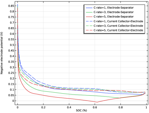
Select the y-axis label checkbox. In the associated text field, type Negative electrode potential (V).
Point Graph 1
1
Right-click Plating Susceptibility, C-rate and choose Point Graph.
2
3
In the Settings window for Point Graph, locate the y-Axis Data section.
4
In the Expression text field, type phis-phil.
5
Click Replace Expression in the upper-right corner of the x-Axis Data section. From the menu, choose Component 1 (comp1) > Lithium-Ion Battery > liion.SOC_cell - Cell state of charge - 1.
6
Click to expand the Legends section. Select the Show legends checkbox.
7
From the Legends list, choose Manual.
8
Filter 1
1
Right-click Point Graph 1 and choose Filter.
2
In the Settings window for Filter, locate the Point Selection section.
3
In the Logical expression for inclusion text field, type liion.cdc1.Icell>0.
Point Graph 2
1
In the Model Builder window, under Results > Plating Susceptibility, C-rate right-click Point Graph 1 and choose Duplicate.
2
In the Settings window for Point Graph, locate the Selection section.
3
Click to select the  Activate Selection toggle button.
4
5
Click  Remove from Selection.
6
7
Click to expand the Coloring and Style section. Find the Line style subsection. From the Line list, choose Dashed.
8
From the Color list, choose Cycle (reset).
9
Locate the Legends section. In the table, enter the following settings:
10
In the Plating Susceptibility, C-rate toolbar, click  Plot.
Lithium Film Thickness, C-rate
1
In the Model Builder window, right-click Plating Susceptibility, C-rate and choose Duplicate.
2
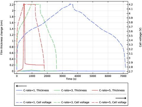
In the Settings window for 1D Plot Group, type Lithium Film Thickness, C-rate in the Label text field.
3
Locate the Plot Settings section. In the x-axis label text field, type Time (s).
4
In the y-axis label text field, type Film thickness change (nm).
Point Graph 1
1
In the Model Builder window, expand the Lithium Film Thickness, C-rate node, then click Point Graph 1.
2
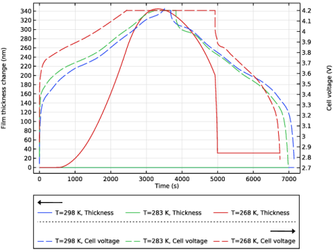
In the Settings window for Point Graph, click Replace Expression in the upper-right corner of the y-Axis Data section. From the menu, choose Component 1 (comp1) > Lithium-Ion Battery > Dissolving–depositing species > liion.sbtot_pce1 - Total film thickness change - m.
3
Locate the y-Axis Data section. From the Unit list, choose nm.
4
Locate the x-Axis Data section. From the Parameter list, choose Time.
5
Click to expand the Legends section. In the table, enter the following settings:
Filter 1
1
In the Model Builder window, expand the Point Graph 1 node.
2
Right-click Filter 1 and choose Delete.
Point Graph 2
In the Model Builder window, right-click Point Graph 2 and choose Delete.
Global 1
1
In the Model Builder window, right-click Lithium Film Thickness, C-rate and choose Global.
2
In the Settings window for Global, locate the y-Axis Data section.
3
4
Click to expand the Coloring and Style section. Find the Line style subsection. From the Line list, choose Dashed.
5
From the Color list, choose Cycle (reset).
6
Click to expand the Legends section. From the Legends list, choose Manual.
7
Lithium Film Thickness, C-rate
1
In the Model Builder window, click Lithium Film Thickness, C-rate.
2
In the Settings window for 1D Plot Group, locate the Plot Settings section.
3
Select the Two y-axes checkbox.
4
Select the Secondary y-axis label checkbox. In the associated text field, type Cell voltage (V).
5
In the table, select the Plot on secondary y-axis checkbox for Global 1.
6
Locate the Legend section. From the Layout list, choose Outside graph axis area.
7
From the Position list, choose Bottom.
8
In the Lithium Film Thickness, C-rate toolbar, click  Plot.
Loss of Lithium Inventory, C-rate
1
In the Model Builder window, right-click Lithium Plating Current, C-rate and choose Duplicate.
2
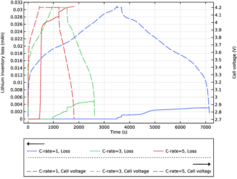
In the Settings window for 1D Plot Group, type Loss of Lithium Inventory, C-rate in the Label text field.
3
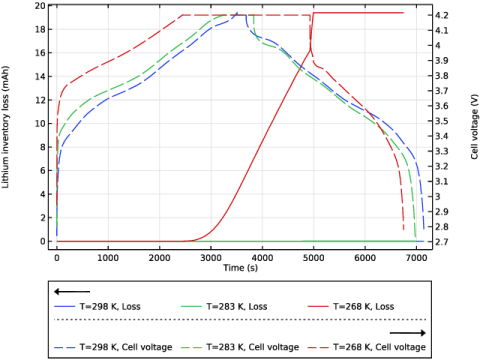
Locate the Plot Settings section. In the y-axis label text field, type Lithium inventory loss (mAh).
4
Locate the Legend section. From the Layout list, choose Outside graph axis area.
5
From the Position list, choose Bottom.
Global 1
1
In the Model Builder window, expand the Loss of Lithium Inventory, C-rate node, then click Global 1.
2
In the Settings window for Global, locate the y-Axis Data section.
3
4
Click to expand the Legends section. In the table, enter the following settings:
5
In the Loss of Lithium Inventory, C-rate toolbar, click  Plot.
Add Study
1
In the Home toolbar, click  Add Study to open the Add Study window.
2
Go to the Add Study window.
Add a new Study with a parametric sweep to study the impact of temperature.
3
Find the Studies subsection. In the Select Study tree, select Preset Studies for Selected Physics Interfaces > Time Dependent with Initialization.
4
Click the Add Study button in the window toolbar.
5
In the Home toolbar, click  Add Study to close the Add Study window.
Study - Temperature
1
In the Settings window for Study, type Study - Temperature in the Label text field.
2
Locate the Study Settings section. Clear the Generate default plots checkbox.
Parametric Sweep
1
In the Study toolbar, click  Parametric Sweep.
2
In the Settings window for Parametric Sweep, locate the Study Settings section.
3
4
Step 2: Time Dependent
1
In the Model Builder window, click Step 2: Time Dependent.
2
In the Settings window for Time Dependent, locate the Study Settings section.
3
In the Output times text field, type range(0,100/C_rate,3600*6/C_rate).
Solution 7 (sol7)
1
In the Study toolbar, click  Show Default Solver.
2
In the Model Builder window, expand the Solution 7 (sol7) node, then click Time-Dependent Solver 1.
3
In the Settings window for Time-Dependent Solver, locate the General section.
4
From the Times to store list, choose Steps taken by solver.
5
Right-click Study - Temperature > Solver Configurations > Solution 7 (sol7) > Time-Dependent Solver 1 and choose Stop Condition.
6
In the Settings window for Stop Condition, locate the Stop Expressions section.
7
8
9
Locate the Output at Stop section. Clear the Add information checkbox.
10
In the Study toolbar, click  Compute.
Results
Plating Susceptibility, Temperature
1
In the Model Builder window, right-click Plating Susceptibility, C-rate and choose Duplicate.
2
In the Settings window for 1D Plot Group, type Plating Susceptibility, Temperature in the Label text field.
3
Locate the Data section. From the Dataset list, choose Study - Temperature/Parametric Solutions 2 (sol9).
Point Graph 1
1
In the Model Builder window, expand the Plating Susceptibility, Temperature node, then click Point Graph 1.
2
In the Settings window for Point Graph, click to expand the Legends section.
3
Point Graph 2
1
In the Model Builder window, click Point Graph 2.
2
In the Settings window for Point Graph, locate the Legends section.
3
4
In the Plating Susceptibility, Temperature toolbar, click  Plot.
Cell Voltage, Temperature
1
In the Model Builder window, right-click Cell Voltage, C-rate and choose Duplicate.
2
In the Settings window for 1D Plot Group, type Cell Voltage, Temperature in the Label text field.
3
Locate the Data section. From the Dataset list, choose Study - Temperature/Parametric Solutions 2 (sol9).
Global 1
1
In the Model Builder window, expand the Cell Voltage, Temperature node, then click Global 1.
2
In the Settings window for Global, click to expand the Legends section.
3
Global 2
1
In the Model Builder window, click Global 2.
2
In the Settings window for Global, locate the Legends section.
3
4
In the Cell Voltage, Temperature toolbar, click  Plot.
Lithium Film Thickness, Temperature
1
In the Model Builder window, right-click Lithium Film Thickness, C-rate and choose Duplicate.
2
In the Settings window for 1D Plot Group, type Lithium Film Thickness, Temperature in the Label text field.
3
Locate the Data section. From the Dataset list, choose Study - Temperature/Parametric Solutions 2 (sol9).
Point Graph 1
1
In the Model Builder window, expand the Lithium Film Thickness, Temperature node, then click Point Graph 1.
2
In the Settings window for Point Graph, click to expand the Legends section.
3
Global 1
1
In the Model Builder window, click Global 1.
2
In the Settings window for Global, locate the Legends section.
3
4
In the Lithium Film Thickness, Temperature toolbar, click  Plot.
Loss of Lithium Inventory, Temperature
1
In the Model Builder window, right-click Loss of Lithium Inventory, C-rate and choose Duplicate.
2
In the Model Builder window, click Loss of Lithium Inventory, C-rate 1.
3
In the Settings window for 1D Plot Group, type Loss of Lithium Inventory, Temperature in the Label text field.
4
Locate the Data section. From the Dataset list, choose Study - Temperature/Parametric Solutions 2 (sol9).
Global 1
1
In the Model Builder window, click Global 1.
2
In the Settings window for Global, locate the Legends section.
3
Global 2
1
In the Model Builder window, click Global 2.
2
In the Settings window for Global, locate the Legends section.
3
4
In the Loss of Lithium Inventory, Temperature toolbar, click  Plot.