| 
|
|
|
|
|
•
|
|
•
|
|
•
|

|
1
|
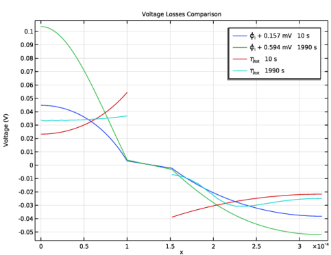
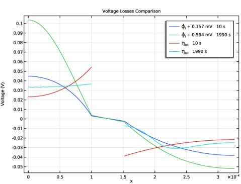
Plot the electrolyte potential profile at the initial stage of the discharge with a bias of 157 mV to get all the plots in the same range of potential.
|
|
2
|
Plot the electrolyte potential profile at the end of the discharge adding a bias of 594 mV, again in order to get the profile in the same scale as the overpotential.
|
|
1
|
|
2
|
|
3
|
Click Add.
|
|
4
|
Click
|
|
5
|
In the Select Study tree, select Preset Studies for Selected Physics Interfaces > Time Dependent with Initialization.
|
|
6
|
Click
|
|
1
|
|
2
|
|
3
|
Click
|
|
4
|
Browse to the model’s Application Libraries folder and double-click the file li_battery_1d_parameters.txt.
|
|
1
|
|
2
|
|
3
|
|
5
|
Click
|
|
1
|
|
2
|
|
3
|
|
4
|
Click
|
|
5
|
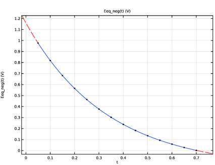
Browse to the model’s Application Libraries folder and double-click the file li_battery_1d_Eeq_neg.txt.
|
|
6
|
Click
|
|
7
|
|
8
|
Locate the Interpolation and Extrapolation section. From the Interpolation list, choose Cubic spline.
|
|
9
|
|
10
|
|
11
|
|
1
|
|
2
|
Go to the Add Material window.
|
|
3
|
|
4
|
Click the Add to Component button in the window toolbar.
|
|
2
|
|
1
|
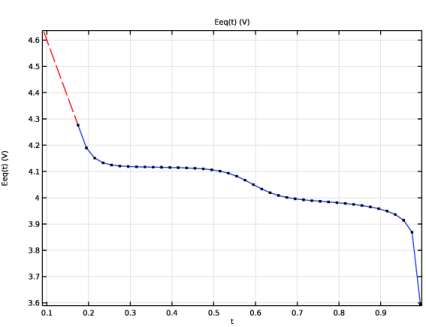
In the Model Builder window, expand the Component 1 (comp1) > Materials > LMO, LiMn2O4 Spinel (Positive, Li-ion Battery) (mat1) > Basic (def) node, then click Interpolation 1 (Eeq, Eeq_inv).
|
|
2
|
|
3
|
Clear the Include right extrapolation checkbox.
|
|
4
|
|
1
|
Go to the Add Material window.
|
|
2
|
In the tree, select Battery > Electrolytes > LiPF6 in 1:2 EC:DMC and p(VdF-HFP) (Polymer, Li-ion Battery).
|
|
3
|
Click the Add to Component button in the window toolbar.
|
|
4
|
|
1
|
Click in the Graphics window and then press Ctrl+A to select all domains.
|
|
2
|
In the Model Builder window, expand the LiPF6 in 1:2 EC:DMC and p(VdF-HFP) (Polymer, Li-ion Battery) (mat2) node.
|
|
1
|
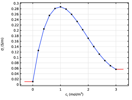
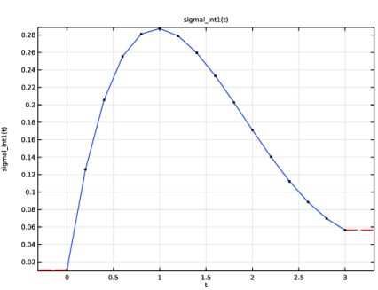
In the Model Builder window, expand the Component 1 (comp1) > Materials > LiPF6 in 1:2 EC:DMC and p(VdF-HFP) (Polymer, Li-ion Battery) (mat2) > Electrolyte conductivity (ionc) node, then click Interpolation 1 (sigmal_int1).
|
|
2
|
|
1
|
|
2
|
|
3
|
|
1
|
In the Model Builder window, under Component 1 (comp1) > Lithium-Ion Battery (liion) click Separator 1.
|
|
2
|
|
3
|
|
1
|
|
3
|
|
4
|
|
5
|
|
6
|
|
7
|
Locate the Effective Transport Parameter Correction section. From the Electrolyte conductivity list, choose User defined. In the fl text field, type epsl_neg^brugg.
|
|
8
|
|
9
|
|
1
|
|
2
|
|
3
|
|
4
|
|
5
|
Locate the Particle Transport Properties section. From the Ds list, choose User defined. In the associated text field, type Ds_neg.
|
|
6
|
|
7
|
Click to expand the Operational SOCs for Initial Cell Charge Distribution section. From the socmin list, choose User defined. From the socmax list, choose User defined.
|
|
1
|
|
2
|
|
3
|
From the Eeq list, choose User defined. In the associated text field, type Eeq_neg(liion.cs_surface/csmax_neg).
|
|
4
|
Locate the Electrode Kinetics section. From the Exchange current density type list, choose Rate constant.
|
|
5
|
|
6
|
|
7
|
|
1
|
|
3
|
|
4
|
|
5
|
|
6
|
|
7
|
Locate the Effective Transport Parameter Correction section. From the Electrolyte conductivity list, choose User defined. In the fl text field, type epsl_pos^brugg.
|
|
8
|
|
9
|
|
1
|
|
2
|
|
3
|
|
4
|
|
5
|
Locate the Particle Transport Properties section. From the Ds list, choose User defined. In the associated text field, type Ds_pos.
|
|
6
|
|
7
|
|
1
|
|
2
|
|
3
|
|
4
|
Locate the Electrode Kinetics section. From the Exchange current density type list, choose Rate constant.
|
|
5
|
|
6
|
|
1
|
|
1
|
|
3
|
|
4
|
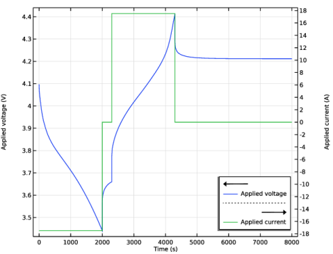
From the list, choose Galvanostatic.
|
|
5
|
|
1
|
|
2
|
|
3
|
|
4
|
|
5
|
|
1
|
|
2
|
|
3
|
|
1
|
|
2
|
|
3
|
|
4
|
|
5
|
|
1
|
|
2
|
|
3
|
Clear the Elapsed time checkbox.
|
|
1
|
In the Model Builder window, under Component 1 (comp1) > Lithium-Ion Battery (liion) click Initial Values 1.
|
|
2
|
|
3
|
|
1
|
|
2
|
|
3
|
|
4
|
|
1
|
|
2
|
|
3
|
|
4
|
|
1
|
In the Model Builder window, under Results click Boundary Electrode Potential with Respect to Ground (liion).
|
|
2
|
|
3
|
|
4
|
|
1
|
|
2
|
|
3
|
|
4
|
|
1
|
|
2
|
|
3
|
|
4
|
|
5
|
|
6
|
|
7
|
|
8
|
|
9
|
|
10
|
|
1
|
|
2
|
|
3
|
|
4
|
|
5
|
Locate the Legends section. In the Legend text field, type \phi<sub>l</sub> + 0.594 mV eval(t,s,4) s.
|
|
1
|
|
2
|
|
3
|
|
4
|
|
5
|
|
1
|
|
2
|
|
3
|
|
4
|
|
5
|
|
1
|
|
2
|
|
3
|
|
4
|
|
1
|
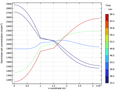
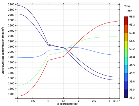
In the Model Builder window, expand the Electrolyte Salt Concentration (liion) node, then click Line Graph 1.
|
|
2
|
|
1
|
|
2
|
|
3
|
|
4
|
|
5
|
|
1
|
|
2
|
|
3
|
|
4
|
|
5
|
|
6
|
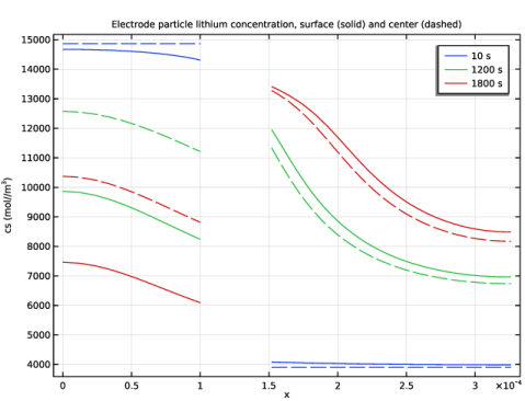
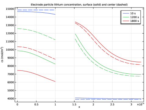
In the Title text area, type Electrode particle lithium concentration, surface (solid) and center (dashed).
|
|
7
|
Locate the Plot Settings section.
|
|
8
|
|
9
|
|
1
|
|
2
|
|
3
|
|
4
|
Click Replace Expression in the upper-right corner of the y-Axis Data section. From the menu, choose Component 1 (comp1) > Lithium-Ion Battery > Particle intercalation > liion.cs_surface - Insertion particle concentration, surface - mol/m³.
|
|
5
|
|
1
|
|
2
|
|
3
|
|
4
|
Click Replace Expression in the upper-right corner of the y-Axis Data section. From the menu, choose Component 1 (comp1) > Lithium-Ion Battery > Particle intercalation > liion.cs_center - Insertion particle concentration, center - mol/m³.
|
|
5
|
Click to expand the Coloring and Style section. Find the Line style subsection. From the Line list, choose Dashed.
|
|
6
|
|
7
|
|
8
|
|
1
|
|
2
|
|
1
|
|
2
|
|
4
|
|
5
|
|
6
|
|
1
|
|
2
|
|
3
|
|
1
|
In the Model Builder window, under Component 1 (comp1) > Lithium-Ion Battery (liion) click Load Cycle 1.
|
|
2
|
|
1
|
|
2
|
Go to the Add Study window.
|
|
3
|
Find the Studies subsection. In the Select Study tree, select Preset Studies for Selected Physics Interfaces > Time Dependent with Initialization.
|
|
4
|
Click the Add Study button in the window toolbar.
|
|
5
|
|
1
|
In the Model Builder window, expand the Study 2 node, then click Step 1: Current Distribution Initialization.
|
|
2
|
In the Settings window for Current Distribution Initialization, locate the Physics and Variables Selection section.
|
|
3
|
Select the Modify model configuration for study step checkbox.
|
|
4
|
|
5
|
Right-click and choose Disable.
|
|
1
|
|
2
|
|
3
|
|
4
|
Locate the Physics and Variables Selection section. Select the Modify model configuration for study step checkbox.
|
|
5
|
|
6
|
Right-click and choose Disable.
|
|
1
|
|
2
|
|
3
|
Click
|
|
1
|
|
2
|
|
3
|
|
4
|
|
5
|
|
6
|
|
7
|
|
8
|
Clear the Generate default plots checkbox.
|
|
9
|
|
1
|
|
2
|
|
3
|
|
1
|
|
3
|
In the Settings window for Point Graph, click Replace Expression in the upper-right corner of the y-Axis Data section. From the menu, choose Component 1 (comp1) > Lithium-Ion Battery > phis - Electric potential - V.
|
|
4
|
|
5
|
|
6
|
|
7
|
|
8
|
|
9
|
|
1
|
|
2
|
|
3
|
|
4
|
|
5
|
Locate the Plot Settings section.
|
|
6
|
|
7
|
|
8
|
|
9
|
|
10
|
|
11
|
|
12
|
|
13
|