
|
|
|
|
•
|
|
•
|
|
•
|

|
•
|
i0,ref is the reference exchange current density.
|
|
•
|
|
•
|
|
•
|

|
1
|
|
2
|
|
3
|
Click Add.
|
|
4
|
|
5
|
Click Add.
|
|
6
|
Click
|
|
7
|
In the Select Study tree, select Preset Studies for Selected Physics Interfaces > Lithium-Ion Battery > Time Dependent with Initialization.
|
|
8
|
Click
|
|
1
|
|
2
|
|
3
|
Click
|
|
4
|
Browse to the model’s Application Libraries folder and double-click the file cu_current_collector_dissolution_parameters.txt.
|
|
1
|
|
2
|
Go to the Add Material window.
|
|
3
|
|
4
|
Click the Add to Component button in the window toolbar.
|
|
5
|
|
6
|
Click the Add to Component button in the window toolbar.
|
|
7
|
|
8
|
Click the Add to Component button in the window toolbar.
|
|
9
|
|
10
|
Click the Add to Component button in the window toolbar.
|
|
11
|
|
1
|
|
2
|
|
3
|
|
4
|
|
1
|
|
2
|
|
3
|
|
4
|
|
5
|
|
1
|
|
2
|
|
3
|
|
4
|
|
5
|
|
1
|
|
2
|
|
3
|
|
4
|
|
5
|
|
1
|
|
2
|
|
3
|
|
4
|
|
5
|
|
6
|
|
7
|
|
1
|
In the Model Builder window, expand the Component 1 (comp1) > Definitions > View 1 node, then click Axis.
|
|
2
|
|
3
|
|
4
|
|
5
|
Click
|
|
6
|
|
1
|
|
2
|
|
1
|
|
2
|
|
1
|
|
2
|
|
1
|
|
2
|
|
1
|
|
2
|
|
1
|
|
2
|
In the Settings window for Explicit, type Copper Current-Collector Boundary in the Label text field.
|
|
3
|
|
1
|
|
2
|
In the Settings window for Explicit, type Aluminum Current-Collector Boundary in the Label text field.
|
|
3
|
|
1
|
|
2
|
In the Settings window for Integration, type Integration - Electrolyte-Filled Domains in the Label text field.
|
|
3
|
|
1
|
In the Model Builder window, under Component 1 (comp1) > Materials click LiPF6 in 1:1 EC:DMC (Liquid, Li-ion Battery) (mat1).
|
|
2
|
|
3
|
Click
|
|
1
|
|
2
|
|
3
|
|
1
|
|
2
|
|
3
|
|
1
|
|
2
|
|
3
|
|
1
|
|
2
|
|
3
|
Click
|
|
4
|
Browse to the model’s Application Libraries folder and double-click the file cu_current_collector_dissolution_variables.txt.
|
|
1
|
In the Model Builder window, under Component 1 (comp1) > Lithium-Ion Battery (liion) click Separator 1.
|
|
2
|
|
3
|
|
1
|
|
2
|
|
3
|
|
1
|
|
2
|
|
3
|
|
1
|
|
2
|
In the Settings window for Porous Electrode, type Porous Electrode - Negative in the Label text field.
|
|
3
|
|
4
|
Locate the Electrolyte Properties section. From the Electrolyte material list, choose LiPF6 in 1:1 EC:DMC (Liquid, Li-ion Battery) (mat1).
|
|
5
|
|
6
|
|
7
|
|
8
|
Locate the Effective Transport Parameter Correction section. From the Electric conductivity list, choose No correction.
|
|
9
|
|
11
|
Clear the Add volume change to electrode volume fraction checkbox.
|
|
12
|
Clear the Subtract volume change from electrolyte volume fraction checkbox.
|
|
1
|
|
2
|
|
3
|
|
4
|
|
1
|
In the Model Builder window, under Component 1 (comp1) > Lithium-Ion Battery (liion) > Porous Electrode - Negative click Porous Electrode Reaction 1.
|
|
2
|
In the Settings window for Porous Electrode Reaction, type Porous Electrode Reaction - Intercalation in the Label text field.
|
|
3
|
|
1
|
|
2
|
In the Settings window for Porous Electrode Reaction, type Porous Electrode Reaction - Copper in the Label text field.
|
|
3
|
Locate the Equilibrium Potential section. From the Eeq list, choose User defined. In the associated text field, type Eeq_Cu+delta_phil.
|
|
4
|
Locate the Electrode Kinetics section. From the Kinetics expression type list, choose Concentration dependent kinetics.
|
|
5
|
|
6
|
|
7
|
|
8
|
|
9
|
In the Stoichiometric coefficients for dissolving–depositing species: table, enter the following settings:
|
|
1
|
|
2
|
In the Settings window for Porous Electrode, type Porous Electrode - Positive in the Label text field.
|
|
3
|
|
4
|
Locate the Electrolyte Properties section. From the Electrolyte material list, choose LiPF6 in 1:1 EC:DMC (Liquid, Li-ion Battery) (mat1).
|
|
5
|
|
6
|
|
7
|
|
8
|
Locate the Effective Transport Parameter Correction section. From the Electric conductivity list, choose No correction.
|
|
1
|
|
2
|
|
3
|
|
4
|
|
1
|
|
2
|
|
3
|
|
1
|
|
2
|
In the Settings window for Internal Electrode Surface, type Internal Electrode Surface - Copper in the Label text field.
|
|
3
|
Locate the Boundary Selection section. From the Selection list, choose Copper Current-Collector Boundary.
|
|
1
|
|
2
|
|
3
|
|
4
|
Locate the Equilibrium Potential section. From the Eeq list, choose User defined. In the associated text field, type Eeq_Cu+delta_phil.
|
|
5
|
Locate the Electrode Kinetics section. From the Kinetics expression type list, choose Concentration dependent kinetics.
|
|
6
|
|
7
|
|
1
|
|
1
|
|
2
|
|
3
|
|
4
|
|
1
|
|
3
|
|
4
|
|
1
|
|
2
|
|
4
|
Click
|
|
6
|
|
7
|
Select the Migration in electric field checkbox.
|
|
8
|
Select the Mass transfer in porous media checkbox.
|
|
9
|
Click to expand the Dependent Variables section. In the Concentrations (mol/m³) table, enter the following settings:
|
|
1
|
In the Model Builder window, under Component 1 (comp1) > Transport of Diluted Species (tds) click Species Charges.
|
|
2
|
|
3
|
|
1
|
|
2
|
|
3
|
|
4
|
|
1
|
|
2
|
In the Settings window for Electrode Surface Coupling, type Electrode Surface Coupling - Copper in the Label text field.
|
|
3
|
Locate the Boundary Selection section. From the Selection list, choose Copper Current-Collector Boundary.
|
|
1
|
In the Model Builder window, expand the Electrode Surface Coupling - Copper node, then click Reaction Coefficients 1.
|
|
2
|
|
3
|
|
4
|
|
1
|
|
2
|
|
3
|
|
1
|
|
2
|
|
3
|
|
4
|
|
5
|
|
1
|
|
2
|
|
3
|
|
1
|
|
2
|
|
3
|
|
1
|
|
2
|
|
3
|
|
4
|
|
5
|
|
1
|
|
2
|
|
3
|
|
1
|
|
2
|
|
3
|
|
1
|
|
2
|
|
3
|
|
4
|
|
5
|
|
1
|
|
2
|
|
3
|
|
1
|
|
2
|
In the Settings window for Porous Electrode Coupling, type Porous Electrode Coupling - Copper in the Label text field.
|
|
3
|
|
1
|
|
2
|
|
3
|
From the iv list, choose Local current source, Porous Electrode Reaction - Copper (liion/pce1/per2).
|
|
4
|
|
1
|
|
2
|
|
3
|
|
4
|
|
1
|
|
2
|
|
3
|
From the list, choose User-controlled mesh.
|
|
1
|
|
2
|
|
3
|
|
5
|
|
1
|
|
2
|
|
3
|
|
4
|
Click
|
|
1
|
|
2
|
|
3
|
Click
|
|
4
|
Click
|
|
1
|
|
2
|
|
3
|
|
4
|
Locate the Physics and Variables Selection section. Select the Modify model configuration for study step checkbox.
|
|
5
|
|
6
|
Right-click and choose Disable.
|
|
1
|
|
2
|
|
3
|
|
1
|
|
2
|
|
3
|
In the Model Builder window, under Study 1 > Solver Configurations > Solution 1 (sol1) click Time-Dependent Solver 1.
|
|
4
|
|
5
|
|
6
|
|
7
|
Right-click Study 1 > Solver Configurations > Solution 1 (sol1) > Time-Dependent Solver 1 and choose Fully Coupled.
|
|
8
|
|
9
|
|
10
|
|
11
|
|
12
|
Click
|
|
14
|
|
15
|
Clear the Add information checkbox.
|
|
16
|
|
1
|
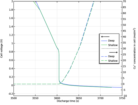
In the Settings window for 1D Plot Group, type Cell Voltage and Concentration in the Label text field.
|
|
2
|
|
3
|
Locate the Plot Settings section.
|
|
4
|
|
5
|
|
6
|
Select the Two y-axes checkbox.
|
|
7
|
Select the Secondary y-axis label checkbox. In the associated text field, type Cu<sup>+</sup> concentration in cell (mol/m<sup>3</sup>).
|
|
8
|
|
9
|
|
10
|
|
11
|
|
12
|
|
13
|
|
14
|
|
15
|
|
16
|
|
1
|
|
2
|
|
3
|
|
1
|
|
2
|
|
4
|
|
5
|
Click to expand the Coloring and Style section. Find the Line style subsection. From the Line list, choose Dashed.
|
|
6
|
|
7
|
|
1
|
|
2
|
|
3
|
|
4
|
|
5
|
|
6
|
Clear the Parameter indicator text field.
|
|
7
|
|
8
|
|
1
|
|
2
|
|
1
|
|
2
|
|
3
|
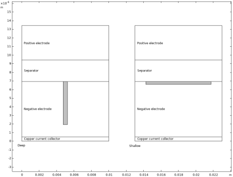
From the Parameter value (w_dent (m),depth_dent (m)) list, choose 1: w_dent=5E-4 m, depth_dent=5E-5 m.
|
|
4
|
|
1
|
|
2
|
|
3
|
|
4
|
From the Parameter value (w_dent (m),depth_dent (m)) list, choose 1: w_dent=5E-4 m, depth_dent=5E-5 m.
|
|
5
|
|
6
|
|
7
|
|
8
|
|
1
|
|
1
|
|
2
|
|
3
|
|
4
|
From the Parameter value (w_dent (m),depth_dent (m)) list, choose 1: w_dent=5E-4 m, depth_dent=5E-5 m.
|
|
5
|
|
6
|
|
7
|
|
8
|
|
1
|
In the Model Builder window, under Results > Cuprous Ion Concentration, Ctrl-click to select Surface 1, Line 1, and Annotation 1.
|
|
2
|
Right-click and choose Duplicate.
|
|
1
|
|
2
|
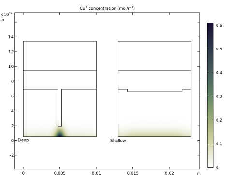
From the Parameter value (w_dent (m),depth_dent (m)) list, choose 2: w_dent=0.0075 m, depth_dent=3.3333E-6 m.
|
|
3
|
Click to expand the Range section. Locate the Coloring and Style section. Clear the Color legend checkbox.
|
|
4
|
|
5
|
|
6
|
|
1
|
|
2
|
|
3
|
From the Parameter value (w_dent (m),depth_dent (m)) list, choose 2: w_dent=0.0075 m, depth_dent=3.3333E-6 m.
|
|
4
|
|
1
|
|
2
|
|
3
|
From the Parameter value (w_dent (m),depth_dent (m)) list, choose 2: w_dent=0.0075 m, depth_dent=3.3333E-6 m.
|
|
4
|
|
5
|
|
1
|
|
2
|
|
3
|
In the Settings window for 2D Plot Group, type Deposited Copper Concentration in the Label text field.
|
|
4
|
Locate the Title section. In the Title text area, type Deposited copper concentration (mol/m<sup>3</sup>).
|
|
1
|
|
2
|
In the Settings window for Surface, click Replace Expression in the upper-right corner of the Expression section. From the menu, choose Component 1 (comp1) > Lithium-Ion Battery > Dissolving–depositing species > liion.c_pce1_CuMetal - Dissolving–depositing species concentration - mol/m³.
|
|
3
|
|
4
|
|
1
|
|
2
|
|
3
|
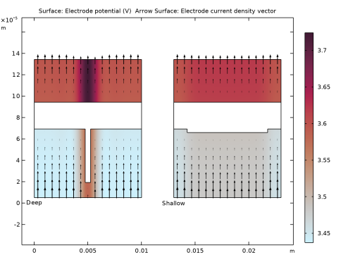
Locate the Title section. In the Title text area, type Surface: Electrode potential (V) Arrow Surface: Electrode current density vector.
|
|
1
|
|
2
|
|
3
|
|
4
|
|
5
|
|
6
|
|
1
|
|
2
|
|
3
|
|
4
|
|
5
|
|
1
|
|
2
|
|
3
|
|
4
|
From the Parameter value (w_dent (m),depth_dent (m)) list, choose 1: w_dent=5E-4 m, depth_dent=5E-5 m.
|
|
5
|
|
6
|
|
7
|
Click Replace Expression in the upper-right corner of the Expression section. From the menu, choose Component 1 (comp1) > Lithium-Ion Battery > liion.Isx,liion.Isy - Electrode current density vector.
|
|
8
|
Locate the Coloring and Style section.
|
|
9
|
|
10
|
|
11
|
|
1
|
|
2
|
|
3
|
From the Parameter value (w_dent (m),depth_dent (m)) list, choose 2: w_dent=0.0075 m, depth_dent=3.3333E-6 m.
|
|
4
|
|
5
|
|
6
|
|
1
|
|
2
|
|
3
|
|
4
|
|
1
|
|
2
|
|
3
|
|
4
|
|
5
|
|
6
|
|
1
|
|
2
|
|
3
|
In the Settings window for 2D Plot Group, type Electrolyte Salt Concentration in the Label text field.
|
|
4
|
Locate the Title section. In the Title text area, type Surface: c<sub>l</sub> concentration (mol/m<sup>3</sup>) Arrow Surface: Electrolyte current density vector.
|
|
1
|
|
2
|
|
3
|
|
4
|
|
5
|
|
1
|
|
2
|
|
3
|
|
4
|
|
1
|
|
2
|
|
3
|
|
4
|
Click Replace Expression in the upper-right corner of the Expression section. From the menu, choose Component 1 (comp1) > Lithium-Ion Battery > liion.Ilx,liion.Ily - Electrolyte current density vector.
|
|
5
|
|
1
|
|
2
|
|
3
|
|
4
|
Click Replace Expression in the upper-right corner of the Expression section. From the menu, choose Component 1 (comp1) > Lithium-Ion Battery > liion.Ilx,liion.Ily - Electrolyte current density vector.
|
|
5
|
|
1
|
|
2
|
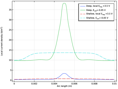
In the Settings window for 1D Plot Group, type Current Collector Dissolution Current in the Label text field.
|
|
3
|
|
4
|
|
1
|
|
2
|
|
3
|
|
4
|
|
5
|
|
6
|
|
8
|
Click Replace Expression in the upper-right corner of the y-Axis Data section. From the menu, choose Component 1 (comp1) > Lithium-Ion Battery > Electrode kinetics > liion.iloc_er1 - Local current density - A/m².
|
|
9
|
|
10
|
|
1
|
|
2
|
|
3
|
|
4
|
Locate the Legends section. In the table, enter the following settings:
|
|
1
|
In the Model Builder window, under Results > Current Collector Dissolution Current, Ctrl-click to select Line Graph 1 and Line Graph 2.
|
|
2
|
Right-click and choose Duplicate.
|
|
1
|
|
2
|
|
3
|
Click to expand the Coloring and Style section. Find the Line style subsection. From the Line list, choose Dashed.
|
|
4
|
Locate the Legends section. In the table, enter the following settings:
|
|
1
|
|
2
|
|
3
|
|
4
|
Locate the Coloring and Style section. Find the Line style subsection. From the Line list, choose Dashed.
|
|
5
|
Locate the Legends section. In the table, enter the following settings:
|
|
6
|
|
1
|
In the Model Builder window, under Results, Ctrl-click to select Average Electrode State of Charge (liion), Electrode Potential with Respect to Ground (liion), Electrode Potential with Respect to Adjacent Reference (liion), Electrolyte Salt Concentration (liion), Separator Current Density Magnitude (liion), and Particle Surface State of Charge (liion).
|
|
2
|
Right-click and choose Delete.
|