|
|
|
 .
.|
•
|
|
•
|
|
•
|
 ,
,
|
1
|
|
2
|
In the Select Physics tree, select Acoustics > Pressure Acoustics > Pressure Acoustics, Time Explicit (pate).
|
|
3
|
Click Add.
|
|
4
|
Click
|
|
5
|
|
6
|
Click
|
|
1
|
|
2
|
|
3
|
|
1
|
|
2
|
|
3
|
|
4
|
|
1
|
|
2
|
|
3
|
Click
|
|
4
|
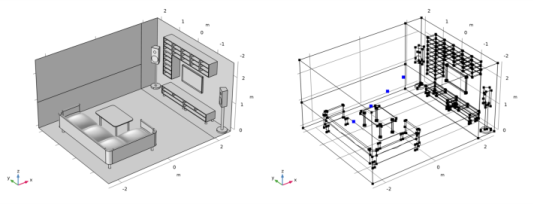
Browse to the model’s Application Libraries folder and double-click the file wave_based_room.mphbin.
|
|
5
|
Click
|
|
6
|
|
1
|
|
2
|
|
3
|
|
4
|
|
5
|
|
6
|
Click
|
|
1
|
|
2
|
|
3
|
|
4
|
Click
|
|
5
|
|
6
|
Click OK.
|
|
1
|
|
2
|
|
3
|
|
4
|
Click
|
|
5
|
|
6
|
Click OK.
|
|
1
|
|
2
|
|
3
|
|
4
|
Click
|
|
5
|
In the Paste Selection dialog, type 116-206, 265-270, 272-274, 277-279, 281-289 in the Selection text field.
|
|
6
|
Click OK.
|
|
1
|
|
2
|
|
3
|
|
4
|
Click
|
|
5
|
|
6
|
Click OK.
|
|
1
|
|
2
|
|
3
|
|
4
|
Click
|
|
5
|
In the Paste Selection dialog, type 79-115, 233-240, 263, 264, 271, 275, 276, 280 in the Selection text field.
|
|
6
|
Click OK.
|
|
1
|
|
2
|
|
3
|
|
4
|
Click
|
|
5
|
|
6
|
Click OK.
|
|
1
|
|
2
|
|
3
|
|
4
|
Click
|
|
5
|
|
6
|
Click OK.
|
|
1
|
|
2
|
|
3
|
|
4
|
Click
|
|
5
|
|
6
|
Click OK.
|
|
1
|
|
2
|
|
3
|
|
4
|
Click
|
|
5
|
|
6
|
Click OK.
|
|
1
|
|
2
|
|
3
|
|
4
|
Click
|
|
5
|
|
6
|
Click OK.
|
|
1
|
|
2
|
|
3
|
|
4
|
Select the All boundaries checkbox.
|
|
1
|
|
2
|
|
3
|
|
5
|
|
1
|
|
2
|
|
3
|
Click
|
|
5
|
|
6
|
|
1
|
|
2
|
|
3
|
Click
|
|
5
|
|
1
|
|
2
|
|
3
|
Click
|
|
5
|
|
1
|
|
2
|
|
3
|
Click
|
|
5
|
|
1
|
|
2
|
|
1
|
|
2
|
|
3
|
|
4
|
|
5
|
|
6
|
Click
|
|
1
|
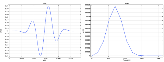
In the Model Builder window, expand the Source Signal Frequency Content node, then click Function 1.
|
|
2
|
|
3
|
|
4
|
|
5
|
|
6
|
Select the Frequency range checkbox.
|
|
7
|
|
8
|
|
1
|
|
2
|
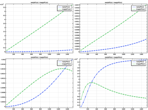
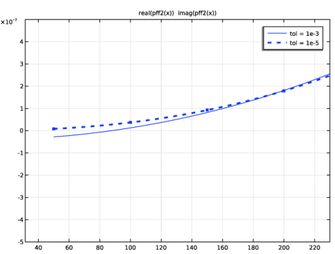
In the Settings window for Partial Fraction Fit, type Partial Fraction Fit - Carpet in the Label text field.
|
|
3
|
|
4
|
Browse to the model’s Application Libraries folder and double-click the file wave_based_room_admittance_carpet.txt.
|
|
5
|
|
6
|
Click
|
|
7
|
Click
|
|
1
|
|
2
|
In the Settings window for Partial Fraction Fit, type Partial Fraction Fit - Ceiling in the Label text field.
|
|
3
|
|
4
|
Browse to the model’s Application Libraries folder and double-click the file wave_based_room_admittance_ceiling.txt.
|
|
5
|
Click
|
|
6
|
Locate the Advanced section. Select the Automatically detect and remove Froissart doublets checkbox.
|
|
7
|
Click
|
|
8
|
Click
|
|
1
|
|
2
|
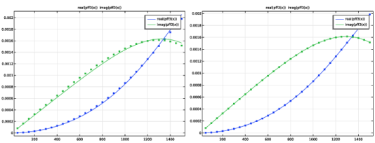
In the Settings window for Partial Fraction Fit, type Partial Fraction Fit - Sofa in the Label text field.
|
|
3
|
|
4
|
Browse to the model’s Application Libraries folder and double-click the file wave_based_room_admittance_sofa.txt.
|
|
5
|
|
6
|
Click
|
|
7
|
Locate the Poles and Residues section. Find the Real residues and poles subsection. Click
|
|
8
|
Click
|
|
9
|
Click
|
|
1
|
|
2
|
In the Settings window for Partial Fraction Fit, type Partial Fraction Fit - Wall in the Label text field.
|
|
3
|
|
4
|
Browse to the model’s Application Libraries folder and double-click the file wave_based_room_admittance_wall.txt.
|
|
5
|
Click
|
|
6
|
Click
|
|
1
|
|
2
|
Go to the Add Material window.
|
|
3
|
|
4
|
Click the Add to Component button in the window toolbar.
|
|
5
|
|
1
|
In the Settings window for Pressure Acoustics, Time Explicit, locate the Model Equation and Solver Settings section.
|
|
2
|
Select the Use accelerated solver formulation checkbox.
|
|
3
|
Clear the Compute residual on GPU checkbox to run the accelerated solver on the CPU.
|
|
1
|
|
2
|
|
4
|
|
5
|
|
6
|
|
1
|
|
2
|
|
3
|
|
4
|
Locate the Impedance section. From the Impedance model list, choose General local reacting (rational approximation).
|
|
5
|
|
6
|
|
7
|
Click
|
|
1
|
|
2
|
|
3
|
|
4
|
Locate the Impedance section. From the Reference list, choose Partial Fraction Fit - Ceiling (pff2).
|
|
5
|
Click
|
|
1
|
|
2
|
|
3
|
|
4
|
|
5
|
Click
|
|
1
|
|
2
|
|
3
|
|
4
|
|
5
|
Click
|
|
1
|
|
2
|
|
3
|
|
1
|
|
2
|
|
3
|
|
1
|
|
2
|
In the Settings window for Free Tetrahedral, click to expand the Element Quality Optimization section.
|
|
3
|
|
4
|
Select the Avoid elements that are too small checkbox.
|
|
1
|
|
2
|
|
3
|
Click the Custom button.
|
|
4
|
|
5
|
|
6
|
|
7
|
Click
|
|
1
|
|
2
|
|
3
|
|
4
|
Click to expand the Store in Output section. In the table, enter the following settings:
|
|
5
|
|
6
|
|
7
|
Click OK.
|
|
8
|
|
9
|
|
10
|
Clear the Generate default plots checkbox.
|
|
11
|
|
1
|
Go to the Probe Table 1 window.
|
|
2
|
Click the Settings button in the window toolbar.
|
|
1
|
|
2
|
|
1
|
|
2
|
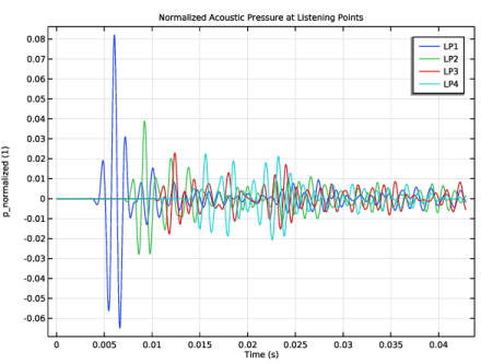
In the Settings window for 1D Plot Group, type Normalized Acoustic Pressure at Listening Points in the Label text field.
|
|
3
|
|
4
|
Locate the Plot Settings section.
|
|
5
|
|
1
|
In the Model Builder window, expand the Normalized Acoustic Pressure at Listening Points node, then click Probe Table Graph 1.
|
|
2
|
|
3
|
|
5
|
|
1
|
|
2
|
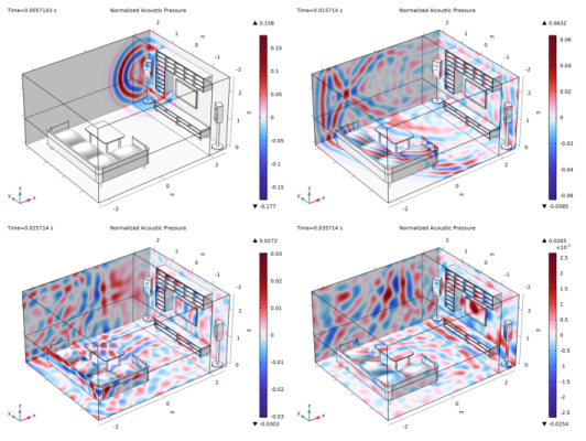
In the Settings window for 3D Plot Group, type Normalized Acoustic Pressure in the Label text field.
|
|
3
|
|
4
|
|
5
|
|
6
|
Select the Show units checkbox.
|
|
1
|
|
2
|
|
3
|
|
4
|
|
5
|
|
1
|
|
2
|
|
3
|
Click
|
|
4
|
|
5
|
Click OK.
|