PDF

Phononic Crystal
Introduction
Phononic crystals are periodic arrangements of macroscopic unit cells that are designed to manipulate elastic-wave propagation. Wave guides, wave filters, and negative refraction lenses are common examples of applications. Unit cells can usually comprise inhomogeneous material properties, arrangements of voids, or resonating elements. When the wavelength of the traveling wave in the crystal approaches twice the characteristic size of the unit cell, Bragg scattering occurs and the crystal behaves as a wave filter in the corresponding frequency range, which is then called the band gap. A similar effect can be obtained with local resonating elements that open band gaps even in the subwavelength regime. Since S and P waves have different equivalent wave speeds, band gaps will open at different frequency ranges for longitudinal and transverse waves.
This model shows how to use the scattered-field formulation to compute the transmission coefficient for impinging plane elastic S and P waves onto a finite-size phononic crystal. The transmission tends to zero in the frequency ranges corresponding to the S- and P-wave band gaps, as predicted by a preliminary study aimed at computing the dispersion relation.
Model Definition
The model comprises two different components:
The crystal is obtained by cutting a square pattern of square holes whose centers are separated by a distance equal to twice the side of the hole itself. The material used is aluminum, with material properties listed in Table 1.
ρ
ν
Different equivalent choices can be made for the geometry of the unit cell. Figure 1 shows the one used in the model.
Figure 1: Unit cell used in the analysis of the dispersion relation.
The assembly of unit cells is thought to be finite in the horizontal direction but infinite in the vertical one. This situation can be simulated numerically by using a monodimensional array of cells in the direction along which the crystal is finite, and periodic conditions in the direction along which the crystal is infinite (see Figure 2). Knowing the desired incident field for which the analysis of the scattering from the crystal is to be performed, the problem can be formulated using the scattered-field formulation, thus solving for the scattered field only.
Note: You can find more information about the scattered-field formulation in the Scattered-Field Formulation for Elastic Waves model. Application Library path: Acoustics_Module/Elastic_Waves/scattered_field_elastic_waves
Figure 2: A strip of 1-by-10 unit cells used to compute reflection and transmission at a surface shared between the phononic crystal and the ambient background material. The top and bottom edges are connected with periodic conditions since the crystal is thought to be infinitely extended in the vertical direction.
Results and Discussion
Figure 3 shows the dispersion relation as computed from the analysis on the unit cell. The computed branches are given color values that are computed based on the longitudinal wave polarization:
(1)
Using such a parameter, Bloch waves dominated by transverse displacements are highlighted in blue, while Bloch waves dominated by longitudinal displacements are highlighted in red. A band gap is opened by Bragg scattering between 0.8 and 1.6 kHz for S waves, while the same happens for P waves between 1.8 and 2.6 kHz. The slope of the dispersion branches in the long-wavelength limit (the wavenumber κ tending to zero) can be used to compute the wave-propagation speed in the crystal,
and the quasistatic homogenized material properties as
where the integrals for computing the homogenized density are performed on the whole volume of the unit cell considering the density inside the holes to be zero, and cS and cP are the computed speeds for S and P waves, respectively.
Figure 3: Dispersion relation.
Figure 4 shows the computed transmission coefficients for incident S and P waves. It illustrates how the crystal works as a mirror for elastic S and P waves in the frequency ranges corresponding to their respective band gaps.
Figure 4: Transmission coefficients for S and P waves as functions of the frequency of the impinging wave.
Figure 5 shows the divergence of the total displacement when a plane P wave is incident from the left on the crystal at a frequency of 2.5 kHz. This illustrates that P waves cannot penetrate into the crystal, which behaves as a mirror.
Figure 5: Total P-wave field obtained when a P wave is incident on the crystal at 2.5 kHz.
Notes About the COMSOL Implementation
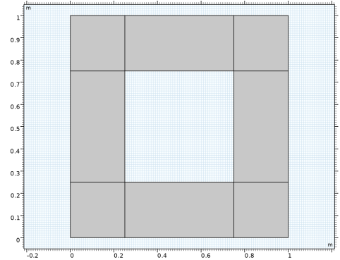
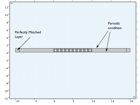
You can add a Periodic Condition boundary condition to the unit cell to simulate an infinite lattice at the computational cost of one cell only. In a similar fashion you can use a Periodic Condition boundary condition even when the crystal is finite in one direction, if you want to consider it infinite in the other directions.
where the total field is seen as the sum of the scattered and background fields. You can instead add a Boundary Load according to
and solve for the scattered field only.
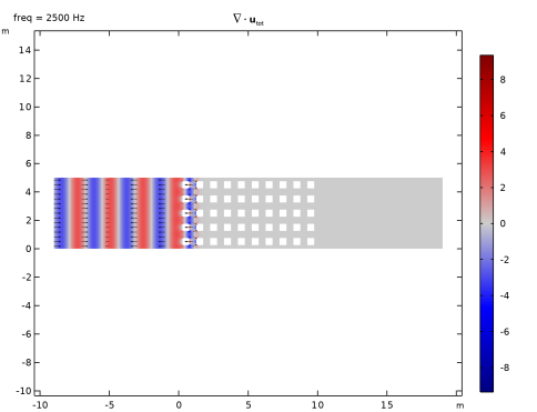
A Perfectly Matched Layer is added to each side of the assembly along the wave propagation direction to truncate the computational domain.
Application Library path: Acoustics_Module/Elastic_Waves/phononic_crystal
Modeling Instructions
From the File menu, choose New.
New
In the New window, click  Model Wizard.
Model Wizard
1
In the Model Wizard window, click  2D.
2
In the Select Physics tree, select Structural Mechanics > Solid Mechanics (solid).
3
Click Add.
4
Click  Study.
5
In the Select Study tree, select General Studies > Eigenfrequency.
6
Part 1
In the Model Builder window, right-click Global Definitions and choose Geometry Parts > 2D Part.
Square 1 (sq1)
1
In the Geometry toolbar, click  Square.
2
In the Settings window for Square, click to expand the Layers section.
3
4
Select the Layers to the left checkbox.
5
Select the Layers to the right checkbox.
6
Select the Layers on top checkbox.
7
Click  Build Selected.
Delete Entities 1 (del1)
1
In the Model Builder window, right-click Part 1 and choose Delete Entities.
2
In the Settings window for Delete Entities, locate the Entities or Objects to Delete section.
3
From the Geometric entity level list, choose Domain.
4
On the object sq1, select Domain 5 only.
5
In the Geometry toolbar, click  Build All.
Geometry 1
Part Instance 1 (pi1)
1
In the Geometry toolbar, click  Part Instance and choose Part 1.
2
In the Settings window for Part Instance, click  Build All Objects.
Global Definitions
Aluminum
1
In the Model Builder window, under Global Definitions right-click Materials and choose Blank Material.
2
In the Settings window for Material, type Aluminum in the Label text field.
3
Click to expand the Material Properties section. In the Material properties tree, select Basic Properties > Density.
4
Click  Add to Material.
5
In the Material properties tree, select Basic Properties > Poisson’s Ratio.
6
Click  Add to Material.
7
In the Material properties tree, select Basic Properties > Young’s Modulus.
8
Click  Add to Material.
9
Locate the Material Contents section. In the table, enter the following settings:
Materials
Material Link 1 (matlnk1)
In the Model Builder window, under Component 1 (comp1) right-click Materials and choose More Materials > Material Link.
Global Definitions
Parameters 1
1
In the Settings window for Parameters, locate the Parameters section.
2
Solid Mechanics (solid)
Periodic Condition 1
1
In the Physics toolbar, click  Boundaries and choose Periodic Condition.
2
3
In the Settings window for Periodic Condition, locate the Periodicity Settings section.
4
From the Type of periodicity list, choose Floquet periodicity.
5
Specify the kF vector as
Periodic Condition 2
1
Right-click Periodic Condition 1 and choose Duplicate.
2
In the Settings window for Periodic Condition, locate the Boundary Selection section.
3
Click  Clear Selection.
4
Definitions
Integration 1 (intop1)
1
In the Definitions toolbar, click  Nonlocal Couplings and choose Integration.
2
Click the  Select All button in the Graphics toolbar.
Mesh 1
Mapped 1
In the Mesh toolbar, click  Mapped.
Size
1
In the Model Builder window, click Size.
2
In the Settings window for Size, locate the Element Size section.
3
From the Predefined list, choose Coarse.
Infinite Crystal
1
In the Model Builder window, click Study 1.
2
In the Settings window for Study, type Infinite Crystal in the Label text field.
Step 1: Eigenfrequency
1
In the Model Builder window, under Infinite Crystal click Step 1: Eigenfrequency.
2
In the Settings window for Eigenfrequency, click to expand the Study Extensions section.
3
Select the Auxiliary sweep checkbox.
4
5
6
In the Study toolbar, click  Compute.
Results
Array 2D 1
1
In the Model Builder window, expand the Results > Datasets node.
2
Right-click Results > Datasets and choose More 2D Datasets > Array 2D.
3
In the Settings window for Array 2D, locate the Array Size section.
4
In the X size text field, type 20.
5
In the Y size text field, type 20.
6
Click to expand the Advanced section. Select the Floquet–Bloch periodicity checkbox.
7
Find the Wave vector subsection. In the X text field, type P*pi.
Mode Shape (solid)
1
In the Model Builder window, expand the Results > Mode Shape (solid) node, then click Mode Shape (solid).
2
In the Settings window for 2D Plot Group, locate the Data section.
3
From the Dataset list, choose Array 2D 1.
4
From the Parameter value (P) list, choose 0.1.
5
From the Eigenfrequency (Hz) list, choose 98.541.
6
Click to expand the Title section. From the Title type list, choose Custom.
7
Find the Solution subsection. Clear the Solution checkbox.
8
Locate the Plot Settings section. Clear the Plot dataset edges checkbox.
Solution Array 1
1
In the Model Builder window, right-click Surface 1 and choose Solution Array.
2
In the Settings window for Solution Array, locate the Data section.
3
From the Parameter selection (P) list, choose From list.
4
In the Parameter values (P) list box, select 0.1.
5
From the Eigenfrequency selection list, choose Manual.
6
In the Eigenfrequency indices (1-6) text field, type 1 2.
7
In the Mode Shape (solid) toolbar, click  Plot.
8
Click the  Zoom Extents button in the Graphics toolbar.
Dispersion Relation
1
In the Results toolbar, click  1D Plot Group.
2
In the Settings window for 1D Plot Group, type Dispersion Relation in the Label text field.
3
Locate the Plot Settings section.
4
Select the x-axis label checkbox. In the associated text field, type \kappa/\pi (1/m).
5
Select the y-axis label checkbox. In the associated text field, type f (kHz).
Global 1
1
Right-click Dispersion Relation and choose Global.
2
In the Settings window for Global, locate the y-Axis Data section.
3
4
Locate the x-Axis Data section. From the Parameter list, choose Expression.
5
In the Expression text field, type P.
6
In the Dispersion Relation toolbar, click  Plot.
Dispersion Relation
1
In the Model Builder window, click Dispersion Relation.
2
In the Settings window for 1D Plot Group, locate the Legend section.
3
Clear the Show legends checkbox.
4
Click to expand the Title section. From the Title type list, choose Label.
Global 1
1
In the Model Builder window, click Global 1.
2
In the Settings window for Global, click to expand the Coloring and Style section.
3
Find the Line style subsection. From the Line list, choose None.
4
Find the Line markers subsection. From the Marker list, choose Asterisk.
5
From the Width list, choose 2.
Color Expression 1
1
Right-click Global 1 and choose Color Expression.
2
In the Settings window for Color Expression, locate the Expression section.
3
In the Expression text field, type intop1(real(u)^2)/intop1(real(solid.disp)^2).
4
Locate the Coloring and Style section. From the Color table list, choose WaveLight.
5
In the Dispersion Relation toolbar, click  Plot.
Long Wavelength Homogenized Properties
1
In the Results toolbar, click  Evaluation Group.
2
In the Settings window for Evaluation Group, type Long Wavelength Homogenized Properties in the Label text field.
3
Locate the Transformation section. Select the Transpose checkbox.
4
Click to expand the Format section. From the Include parameters list, choose Off.
S Waves
1
Right-click Long Wavelength Homogenized Properties and choose Global Evaluation.
2
In the Settings window for Global Evaluation, type S Waves in the Label text field.
3
Locate the Data section. From the Dataset list, choose Infinite Crystal/Solution 1 (sol1).
4
From the Parameter selection (P) list, choose From list.
5
In the Parameter values (P) list box, select 0.02.
6
From the Eigenfrequency selection list, choose First.
7
Locate the Expressions section. In the table, enter the following settings:
P Waves
1
Right-click S Waves and choose Duplicate.
2
In the Settings window for Global Evaluation, type P Waves in the Label text field.
3
Locate the Data section. From the Eigenfrequency selection list, choose Manual.
4
In the Eigenfrequency indices (1-6) text field, type 2.
5
Locate the Expressions section. In the table, enter the following settings:
6
In the Long Wavelength Homogenized Properties toolbar, click  Evaluate.
Add Component
Right-click P Waves and choose 2D.
Unit Cell
In the Settings window for Component, type Unit Cell in the Label text field.
Finite Crystal
1
In the Model Builder window, click Component 2 (comp2).
2
In the Settings window for Component, type Finite Crystal in the Label text field.
Geometry 2
Part Instance 1 (pi1)
1
In the Geometry toolbar, click  Part Instance and choose Part 1.
2
In the Settings window for Part Instance, click  Build Selected.
Add Physics
1
In the Physics toolbar, click  Add Physics to open the Add Physics window.
2
Go to the Add Physics window.
3
In the tree, select Recently Used > Solid Mechanics (solid).
4
Click the Add to Finite Crystal button in the window toolbar.
5
In the Physics toolbar, click  Add Physics to close the Add Physics window.
Definitions (comp2)
Incident P Wave
1
In the Model Builder window, under Finite Crystal (comp2) right-click Definitions and choose Variables.
2
In the Settings window for Variables, type Incident P Wave in the Label text field.
3
Locate the Variables section. In the table, enter the following settings:
Solid Mechanics 2 (solid2)
Periodic Condition 1
1
In the Physics toolbar, click  Boundaries and choose Periodic Condition.
2
Boundary Load 1
1
In the Physics toolbar, click  Boundaries and choose Boundary Load.
2
3
In the Settings window for Boundary Load, locate the Force section.
4
Specify the fA vector as
Geometry 2
Array 1 (arr1)
1
In the Geometry toolbar, click  Transforms and choose Array.
2
In the Settings window for Array, locate the Size section.
3
In the x size text field, type 10.
4
Locate the Displacement section. In the x text field, type 1.
5
Click the  Select All button in the Graphics toolbar.
6
Click  Build Selected.
7
Click the  Zoom Extents button in the Graphics toolbar.
Rectangle 1 (r1)
1
In the Geometry toolbar, click  Rectangle.
2
In the Settings window for Rectangle, locate the Size and Shape section.
3
In the Width text field, type 10.
4
Locate the Position section. In the x text field, type -10.
5
Click to expand the Layers section. In the table, enter the following settings:
6
Select the Layers to the left checkbox.
7
Clear the Layers on bottom checkbox.
8
Click  Build Selected.
9
Click the  Zoom Extents button in the Graphics toolbar.
Rectangle 2 (r2)
1
Right-click Rectangle 1 (r1) and choose Duplicate.
2
In the Settings window for Rectangle, locate the Position section.
3
In the x text field, type 10.
4
Locate the Layers section. Clear the Layers to the left checkbox.
5
Select the Layers to the right checkbox.
6
Click  Build Selected.
7
Click the  Zoom Extents button in the Graphics toolbar.
Definitions (comp2)
Perfectly Matched Layer 1 (pml1)
1
In the Definitions toolbar, click  Perfectly Matched Layer.
2
Scattered Intensity
1
In the Definitions toolbar, click  Nonlocal Couplings and choose Average.
2
In the Settings window for Average, locate the Source Selection section.
3
From the Geometric entity level list, choose Boundary.
4
5
In the Label text field, type Scattered Intensity.
Materials
Material Link 2 (matlnk2)
In the Model Builder window, under Finite Crystal (comp2) right-click Materials and choose More Materials > Material Link.
Solid Mechanics 2 (solid2)
Periodic Condition 1
Select Boundaries 2, 3, 5, 6, 8, 13, 15, 20, 22, 27, 29, 34, 36, 41, 43, 48, 50, 55, 57, 62, 64, 69, 71, 76, 78, 83, 85, 90, 92, 97, 99, 104, 106, 111, 113, 118, 120, 125, 127, 132, 134, 139, 141, 146, 148, 153, 155, 160, 162, 167, 169, 174, 176, 181, 183, 188, 190, 195, 197, 202, 204, 209, 211, 216, 218, 221, 223, and 224 only.
Mesh 2
Mapped 1
1
In the Mesh toolbar, click  Mapped.
2
In the Settings window for Mapped, locate the Domain Selection section.
3
From the Geometric entity level list, choose Domain.
4
Free Triangular 1
In the Mesh toolbar, click  Free Triangular.
Size
1
In the Model Builder window, click Size.
2
In the Settings window for Size, locate the Element Size section.
3
From the Predefined list, choose Extremely fine.
4
Click to expand the Element Size Parameters section. In the Maximum element size text field, type 0.1.
5
Click  Build All.
Add Study
1
In the Study toolbar, click  Add Study to open the Add Study window.
2
Go to the Add Study window.
3
Find the Studies subsection. In the Select Study tree, select General Studies > Frequency Domain.
4
Click the Add Study button in the window toolbar.
5
In the Study toolbar, click  Add Study to close the Add Study window.
Infinite Crystal
Step 1: Eigenfrequency
1
In the Settings window for Eigenfrequency, locate the Physics and Variables Selection section.
2
Select the Modify model configuration for study step checkbox.
3
In the tree, select Finite Crystal (comp2) > Solid Mechanics 2 (solid2).
4
Click  Disable in Model.
Infinite Crystal
In the Model Builder window, collapse the Infinite Crystal node.
Finite Crystal: P Wave
1
In the Model Builder window, click Study 2.
2
In the Settings window for Study, type Finite Crystal: P Wave in the Label text field.
3
Locate the Study Settings section. Clear the Generate default plots checkbox.
Step 1: Frequency Domain
1
In the Model Builder window, under Finite Crystal: P Wave click Step 1: Frequency Domain.
2
In the Settings window for Frequency Domain, locate the Study Settings section.
3
In the Frequencies text field, type range(100, 5, 2500 ).
4
Locate the Physics and Variables Selection section. Select the Modify model configuration for study step checkbox.
5
In the tree, select Unit Cell (comp1) > Solid Mechanics (solid).
6
Click  Disable in Model.
7
In the Study toolbar, click  Compute.
Results
Array 2D 2
1
In the Results toolbar, click  More Datasets and choose Array 2D.
2
In the Settings window for Array 2D, locate the Array Size section.
3
In the Y size text field, type 5.
4
Locate the Data section. From the Dataset list, choose Finite Crystal: P Wave/Solution 2 (sol2).
Selection
1
In the Results toolbar, click  Attributes and choose Selection.
2
In the Settings window for Selection, locate the Geometric Entity Selection section.
3
From the Geometric entity level list, choose Domain.
4
Click the  Select All button in the Graphics toolbar.
5
P Wave Incident: P Wave Scattered
1
In the Results toolbar, click  2D Plot Group.
2
In the Settings window for 2D Plot Group, type P Wave Incident: P Wave Scattered in the Label text field.
3
Locate the Data section. From the Dataset list, choose Array 2D 2.
4
Locate the Title section. From the Title type list, choose Manual.
5
In the Title text area, type \$ \nabla \cdot \mathbf{u}_\mathrm{tot} \$.
6
In the Parameter indicator text field, type freq = eval(freq) Hz.
7
Locate the Plot Settings section. Clear the Plot dataset edges checkbox.
Surface 1
1
Right-click P Wave Incident: P Wave Scattered and choose Surface.
2
In the Settings window for Surface, locate the Expression section.
3
In the Expression text field, type d(u2+uP,x)+d(v2+vP,y).
4
Locate the Coloring and Style section. From the Color table list, choose WaveClassic.
5
From the Scale list, choose Linear symmetric.
6
In the P Wave Incident: P Wave Scattered toolbar, click  Plot.
Arrow Surface 1
1
In the Model Builder window, right-click P Wave Incident: P Wave Scattered and choose Arrow Surface.
2
In the Settings window for Arrow Surface, locate the Expression section.
3
In the x-component text field, type u2+uP.
4
In the y-component text field, type v2+vP.
5
Locate the Coloring and Style section. From the Arrow length list, choose Logarithmic.
6
From the Color list, choose Black.
P Wave Incident: P Wave Scattered
1
In the Model Builder window, click P Wave Incident: P Wave Scattered.
2
In the P Wave Incident: P Wave Scattered toolbar, click  Plot.
P Wave Incident: S Wave Scattered
1
Right-click P Wave Incident: P Wave Scattered and choose Duplicate.
2
In the Model Builder window, click P Wave Incident: P Wave Scattered 1.
3
In the Settings window for 2D Plot Group, type P Wave Incident: S Wave Scattered in the Label text field.
4
Locate the Title section. In the Title text area, type \$ \nabla \times \mathbf{u}_\mathrm{tot} \$.
Surface 1
1
In the Model Builder window, click Surface 1.
2
In the Settings window for Surface, locate the Expression section.
3
In the Expression text field, type -d(u2+uP,y)+d(v2+vP,x).
4
In the P Wave Incident: S Wave Scattered toolbar, click  Plot.
Transmission Coefficient
1
In the Results toolbar, click  1D Plot Group.
2
In the Settings window for 1D Plot Group, type Transmission Coefficient in the Label text field.
3
Locate the Data section. From the Dataset list, choose Finite Crystal: P Wave/Solution 2 (sol2).
4
Locate the Title section. From the Title type list, choose Label.
5
Locate the Plot Settings section.
6
Select the x-axis label checkbox. In the associated text field, type f (kHz).
7
Select the y-axis label checkbox. In the associated text field, type (1).
P Wave
1
Right-click Transmission Coefficient and choose Global.
2
In the Settings window for Global, type P Wave in the Label text field.
3
Locate the y-Axis Data section. In the table, enter the following settings:
4
Locate the x-Axis Data section. From the Unit list, choose kHz.
5
Locate the Coloring and Style section. From the Width list, choose 2.
6
Click to expand the Legends section. Find the Include subsection. Clear the Solution checkbox.
7
Clear the Description checkbox.
8
Select the Label checkbox.
9
In the Transmission Coefficient toolbar, click  Plot.
Finite Crystal: P Wave
In the Model Builder window, collapse the Finite Crystal: P Wave node.
Add Study
1
In the Study toolbar, click  Add Study to open the Add Study window.
2
Go to the Add Study window.
3
Find the Studies subsection. In the Select Study tree, select General Studies > Frequency Domain.
4
Click the Add Study button in the window toolbar.
5
In the Study toolbar, click  Add Study to close the Add Study window.
Finite Crystal: S Wave
1
In the Settings window for Study, type Finite Crystal: S Wave in the Label text field.
2
Locate the Study Settings section. Clear the Generate default plots checkbox.
Step 1: Frequency Domain
1
In the Model Builder window, under Finite Crystal: S Wave click Step 1: Frequency Domain.
2
In the Settings window for Frequency Domain, locate the Study Settings section.
3
In the Frequencies text field, type range(100, 5, 2500).
4
Locate the Physics and Variables Selection section. Select the Modify model configuration for study step checkbox.
5
In the tree, select Unit Cell (comp1) > Solid Mechanics (solid).
6
Click  Disable in Model.
Definitions (comp2)
Incident S Wave
1
In the Model Builder window, under Finite Crystal (comp2) right-click Definitions and choose Variables.
2
In the Settings window for Variables, type Incident S Wave in the Label text field.
3
Locate the Variables section. In the table, enter the following settings:
Solid Mechanics 2 (solid2)
1
In the Model Builder window, under Finite Crystal (comp2) click Solid Mechanics 2 (solid2).
2
In the Settings window for Solid Mechanics, click to expand the Typical Wave Speed for Perfectly Matched Layers section.
3
In the cref text field, type solid2.cs.
Boundary Load: P Wave
1
In the Model Builder window, under Finite Crystal (comp2) > Solid Mechanics 2 (solid2) click Boundary Load 1.
2
In the Settings window for Boundary Load, type Boundary Load: P Wave in the Label text field.
Boundary Load: S Wave
1
Right-click Boundary Load: P Wave and choose Duplicate.
2
In the Settings window for Boundary Load, type Boundary Load: S Wave in the Label text field.
3
Locate the Force section. Specify the fA vector as
Finite Crystal: P Wave
Step 1: Frequency Domain
1
In the Model Builder window, expand the Finite Crystal: P Wave node, then click Step 1: Frequency Domain.
2
In the Settings window for Frequency Domain, locate the Physics and Variables Selection section.
3
In the tree, select Finite Crystal (comp2) > Solid Mechanics 2 (solid2) > Boundary Load: S Wave.
4
Click  Disable.
Finite Crystal: S Wave
1
In the Model Builder window, under Finite Crystal: S Wave click Step 1: Frequency Domain.
2
In the Settings window for Frequency Domain, locate the Physics and Variables Selection section.
3
In the tree, select Finite Crystal (comp2) > Solid Mechanics 2 (solid2) > Boundary Load: P Wave.
4
Click  Disable.
5
In the Study toolbar, click  Compute.
Results
Array 2D 3
1
In the Model Builder window, under Results > Datasets right-click Array 2D 2 and choose Duplicate.
2
In the Settings window for Array 2D, locate the Data section.
3
From the Dataset list, choose Finite Crystal: S Wave/Solution 3 (sol3).
S Wave Incident: P Wave Scattered
1
In the Model Builder window, right-click P Wave Incident: P Wave Scattered and choose Duplicate.
2
In the Settings window for 2D Plot Group, type S Wave Incident: P Wave Scattered in the Label text field.
3
Locate the Data section. From the Dataset list, choose Array 2D 3.
4
From the Parameter value (freq (Hz)) list, choose 1200.
Surface 1
1
In the Model Builder window, expand the S Wave Incident: P Wave Scattered node, then click Surface 1.
2
In the Settings window for Surface, locate the Expression section.
3
In the Expression text field, type d(u2+uS,x)+d(v2+vS,y).
Arrow Surface 1
1
In the Model Builder window, click Arrow Surface 1.
2
In the Settings window for Arrow Surface, locate the Expression section.
3
In the x-component text field, type u2+uS.
4
In the y-component text field, type v2+vS.
5
In the S Wave Incident: P Wave Scattered toolbar, click  Plot.
S Wave Incident: S Wave Scattered
1
In the Model Builder window, right-click P Wave Incident: S Wave Scattered and choose Duplicate.
2
In the Settings window for 2D Plot Group, type S Wave Incident: S Wave Scattered in the Label text field.
3
Locate the Data section. From the Dataset list, choose Array 2D 3.
4
From the Parameter value (freq (Hz)) list, choose 1200.
Surface 1
1
In the Model Builder window, expand the S Wave Incident: S Wave Scattered node, then click Surface 1.
2
In the Settings window for Surface, locate the Expression section.
3
In the Expression text field, type -d(u2+uS,y)+d(v2+vS,x).
Arrow Surface 1
1
In the Model Builder window, click Arrow Surface 1.
2
In the Settings window for Arrow Surface, locate the Expression section.
3
In the x-component text field, type u2+uS.
4
In the y-component text field, type v2+vS.
5
In the S Wave Incident: S Wave Scattered toolbar, click  Plot.
S Wave
1
In the Model Builder window, right-click P Wave and choose Duplicate.
2
In the Settings window for Global, type S Wave in the Label text field.
3
Locate the Data section. From the Dataset list, choose Finite Crystal: S Wave/Solution 3 (sol3).
4
Locate the y-Axis Data section. In the table, enter the following settings:
5
In the Transmission Coefficient toolbar, click  Plot.
P Wave Incident: P Wave Scattered
Click the  Zoom Extents button in the Graphics toolbar.