PDF

Scattered-Field Formulation for Elastic Waves
Introduction
This model showcases how to solve for the scattered field when knowing the incident field for three different types of scatterer, that is, an infinitely rigid one, a cavity, and an elastic inclusion.
This formulation can be useful when the scatterer is in the far field of the source, so that the probing wave resembles a plane wave. In such cases, including the source would require a huge computational domain to be meshed. Both P and S plane waves are thus used as incident fields in the model.
Moreover, the model shows how to numerically compute the field emitted by a point source and how to use the obtained solution as the known incident field for a subsequent study solving the scattering problem.
Model Definition
The model geometry consists of an obstacle shaped as an infinite cylinder embedded in an infinite background consisting of an elastic material. Focusing the attention on P and S waves, the plane-strain assumption holds and you can simply model a plane perpendicular to the axis of the cylindrical object. The infinite extension of the background elastic material can be simulated by adopting a finite computational domain truncated with perfectly matched layers. The radius of the obstacle is arbitrarily selected to be unitary, and the frequency is selected such that the wavelength of the P waves is unitary too.
Domain Equations
The field equation for the background field reads
The field equation for the total field reads
where the elasticity tensor and the density are equal to the those of the background outside the scatterer and equal to those of the obstacle inside it. Defining the scattered field as
and subtracting the field equation for the background from that of the total gives
outside the scatterer, while
inside it. This equation can be rewritten as
Thus, one can solve for the scattered field by including in the standard elastodynamic problem a body force, an initial strain, and an initial stress according to
Boundary Conditions
An infinitely rigid obstacle is one for which no displacements can occur and it can therefore be simulated using a homogeneous Dirichlet (fixed) boundary condition:
Rewriting this equation in terms of the scattered field, one obtains
A cavity is such that its boundaries are stress free, which corresponds to a homogeneous Neumann condition:
Thus
Results
Figure 1 shows the displacement magnitude of the scattered field as obtained when a unitary-amplitude plane wave impinges on the three different types of obstacles.
Figure 1: Displacement magnitude of the scattered field for unitary-amplitude incident S (top row) and P (bottom row) plane waves for different types of obstacles.
The top row is the field obtained for an incident S wave, while the bottom row shows the scattered field for a P wave. Exploiting the fact that S waves are divergence free and P waves are curl free, the scattered field can be separated into a P and an S contribution for each analyzed case.
Figure 2: P wave scattered for incident S (top row) and P (bottom row) plane waves for different types of obstacles.
Figure 2 shows the scattered P wave, while Figure 3 shows the scattered S wave.
Figure 3: S wave scattered for incident S (top row) and P (bottom row) plane waves for different types of obstacles.
Adding the known incident field to the solved scattered field gives the total field shown in Figure 4, Figure 5, and Figure 6 in terms of the displacement magnitude, P wave, and S wave, respectively.
Figure 4: Total displacement magnitude for unitary-amplitude incident S (top row) and P (bottom row) plane waves for different types of obstacles.
Figure 5: Total P wave field obtained for unitary-amplitude incident S (top row) and P (bottom row) plane waves for different types of obstacles.
Figure 6: Total S wave field obtained for unitary-amplitude incident S (top row) and P (bottom row) plane waves for different types of obstacles.
Figure 7 shows instead the field produced by a point source in a homogeneous infinitely extended medium. This is used as an incident field to find the fields shown in Figure 8. In Figure 9, the total field obtained summing the scattered field and the incident field shown in Figure 7 is compared to the solution of the same problem solved without the scattered field formulation (SFF) using the point source along with the field equation and boundary conditions for the total field directly.
Figure 7: Point source in terms of displacement magnitude and P and S waves.
Figure 8: Scattered field produced by a point source for different types of obstacles.
Figure 9: Total field obtained with a point source and different types of obstacles. The top row shows the results obtained without the scattered field formulation (SFF), while the bottom row shows the results obtained summing the incident field to the scattered solved with the SFF.
Application Library path: Acoustics_Module/Elastic_Waves/scattered_field_elastic_waves
Modeling Instructions
From the File menu, choose New.
New
In the New window, click  Model Wizard.
Model Wizard
1
In the Model Wizard window, click  2D.
2
In the Select Physics tree, select Structural Mechanics > Solid Mechanics (solid).
3
Click Add.
4
Click  Study.
5
In the Select Study tree, select General Studies > Frequency Domain.
6
Global Definitions
Material Parameters
1
In the Model Builder window, under Global Definitions click Parameters 1.
2
In the Settings window for Parameters, type Material Parameters in the Label text field.
3
Locate the Parameters section. In the table, enter the following settings:
P Wave Parameters
1
In the Home toolbar, click  Parameters and choose Add > Parameters.
2
In the Settings window for Parameters, type P Wave Parameters in the Label text field.
3
Locate the Parameters section. In the table, enter the following settings:
S Wave Parameters
1
In the Home toolbar, click  Parameters and choose Add > Parameters.
2
In the Settings window for Parameters, type S Wave Parameters in the Label text field.
3
Locate the Parameters section. In the table, enter the following settings:
Geometrical Parameters
1
In the Home toolbar, click  Parameters and choose Add > Parameters.
2
In the Settings window for Parameters, type Geometrical Parameters in the Label text field.
3
Locate the Parameters section. In the table, enter the following settings:
Geometry 1
Circle 1 (c1)
1
In the Geometry toolbar, click  Circle.
2
In the Settings window for Circle, locate the Size and Shape section.
3
In the Radius text field, type R.
4
Click to expand the Layers section. In the table, enter the following settings:
5
Click  Build Selected.
Add more copies of the computational domain in order to solve for cavity inclusion, infinitely rigid obstacle, and elastic inclusion at the same time.
Array 1 (arr1)
1
In the Geometry toolbar, click  Transforms and choose Array.
2
3
In the Settings window for Array, locate the Size section.
4
From the Array type list, choose Linear.
5
In the Size text field, type 3.
6
Locate the Displacement section. In the x text field, type 2*(R+r_o).
7
Click  Build Selected.
8
Click the  Zoom Extents button in the Graphics toolbar.
Delete Entities 1 (del1)
1
In the Model Builder window, right-click Geometry 1 and choose Delete Entities.
2
In the Settings window for Delete Entities, locate the Entities or Objects to Delete section.
3
From the Geometric entity level list, choose Domain.
4
On the object arr1(1), select Domain 9 only.
5
On the object arr1(2), select Domain 9 only.
6
Click  Build All Objects.
Definitions
Perfectly Matched Layer 1 (pml1)
1
In the Model Builder window, expand the Component 1 (comp1) > Definitions node.
2
Right-click Definitions and choose Perfectly Matched Layer.
3
4
In the Settings window for Perfectly Matched Layer, locate the Geometry section.
5
From the Type list, choose Cylindrical.
Artificial Domains
Perfectly Matched Layer 2 (pml2)
1
In the Definitions toolbar, click  Perfectly Matched Layer.
2
3
In the Settings window for Perfectly Matched Layer, locate the Geometry section.
4
From the Type list, choose Cylindrical.
Perfectly Matched Layer 3 (pml3)
1
In the Definitions toolbar, click  Perfectly Matched Layer.
2
3
In the Settings window for Perfectly Matched Layer, locate the Geometry section.
4
From the Type list, choose Cylindrical.
First, set up the simulation for an incident P wave.
Definitions
Incident P Wave
1
In the Model Builder window, under Component 1 (comp1) right-click Definitions and choose Variables.
2
In the Settings window for Variables, type Incident P Wave in the Label text field.
3
Locate the Variables section. In the table, enter the following settings:
The internal variable phase is used to synchronize the incident field with the solved scattered field in plots and animations over the dynamic data extension.
Solid Mechanics (solid)
Background Material
1
In the Model Builder window, under Component 1 (comp1) > Solid Mechanics (solid) click Linear Elastic Material 1.
2
In the Settings window for Linear Elastic Material, type Background Material in the Label text field.
3
Locate the Linear Elastic Material section. From the Specify list, choose Pressure-wave and shear-wave speeds.
4
From the cp list, choose User defined. In the associated text field, type cP.
5
From the cs list, choose User defined. In the associated text field, type cS.
6
From the ρ list, choose User defined. In the associated text field, type rho.
Add the boundary condition for a cavity inclusion.
Cavity Inclusion, P Wave
1
In the Physics toolbar, click  Boundaries and choose Boundary Load.
2
In the Settings window for Boundary Load, type Cavity Inclusion, P Wave in the Label text field.
3
4
Locate the Force section. Specify the fA vector as
Now add the boundary condition for an infinitely rigid inclusion.
Infinitely Rigid Inclusion, P Wave
1
In the Physics toolbar, click  Boundaries and choose Prescribed Displacement.
2
In the Settings window for Prescribed Displacement, type Infinitely Rigid Inclusion, P Wave in the Label text field.
3
4
Locate the Prescribed Displacement section. From the Displacement in x direction list, choose Prescribed.
5
In the u0x text field, type -uP.
6
From the Displacement in y direction list, choose Prescribed.
7
In the u0y text field, type -vP.
Finally, set up the domain equation for the elastic inclusion.
Elastic Inclusion, P Wave
1
In the Physics toolbar, click  Domains and choose Linear Elastic Material.
2
In the Settings window for Linear Elastic Material, type Elastic Inclusion, P Wave in the Label text field.
3
4
Locate the Linear Elastic Material section. From the Specify list, choose Lamé parameters.
5
From the λ list, choose User defined. In the associated text field, type lambLame_o.
6
From the μ list, choose User defined. In the associated text field, type muLame_o.
7
From the ρ list, choose User defined. In the associated text field, type rho_o.
Add the initial stress and strain computed from the background field.
Initial Stress and Strain 1
1
In the Physics toolbar, click  Attributes and choose Initial Stress and Strain.
2
In the Settings window for Initial Stress and Strain, locate the Initial Stress and Strain section.
3
Specify the S0 matrix as
4
Specify the ε0 matrix as
Add also the body force.
Body Load (Elastic Inclusion), P Wave
1
In the Physics toolbar, click  Domains and choose Body Load.
2
In the Settings window for Body Load, type Body Load (Elastic Inclusion), P Wave in the Label text field.
3
4
Locate the Force section. Specify the fV vector as
Mesh 1
Mapped 1
1
In the Mesh toolbar, click  Mapped.
2
In the Settings window for Mapped, locate the Domain Selection section.
3
From the Geometric entity level list, choose Domain.
4
Free Triangular 1
In the Mesh toolbar, click  Free Triangular.
Size
1
In the Model Builder window, click Size.
2
In the Settings window for Size, locate the Element Size section.
3
Click the Custom button.
4
Locate the Element Size Parameters section. In the Maximum element size text field, type wlengthS/6.
5
In the Minimum element size text field, type wlengthS/8.
6
Click  Build All.
P Wave
1
In the Model Builder window, click Study 1.
2
In the Settings window for Study, type P Wave in the Label text field.
3
Locate the Study Settings section. Clear the Generate default plots checkbox.
Step 1: Frequency Domain
1
In the Model Builder window, under P Wave click Step 1: Frequency Domain.
2
In the Settings window for Frequency Domain, locate the Study Settings section.
3
In the Frequencies text field, type omega/2/pi[rad].
P Wave
1
In the Model Builder window, expand the Results node.
2
Right-click P Wave and choose Compute.
Results
Scattered u Field
1
In the Results toolbar, click  2D Plot Group.
2
In the Settings window for 2D Plot Group, type Scattered u Field in the Label text field.
3
Click to expand the Title section. From the Title type list, choose Manual.
4
In the Title text area, type Displacement Field, X-component.
5
Clear the Parameter indicator text field.
6
Locate the Plot Settings section. Clear the Plot dataset edges checkbox.
Surface 1
1
Right-click Scattered u Field and choose Surface.
2
In the Settings window for Surface, locate the Expression section.
3
In the Expression text field, type u.
4
Locate the Coloring and Style section. From the Scale list, choose Linear symmetric.
Selection 1
1
Right-click Surface 1 and choose Selection.
2
Scattered u Field
In the Model Builder window, under Results click Scattered u Field.
Table Annotation 1
1
In the Scattered u Field toolbar, click  More Plots and choose Table Annotation.
2
In the Settings window for Table Annotation, locate the Data section.
3
From the Source list, choose Local table.
4
5
In the Scattered u Field toolbar, click  Plot.
6
Locate the Coloring and Style section. From the Anchor point list, choose Center.
7
Clear the Show point checkbox.
Surface 1
1
Click the  Zoom Extents button in the Graphics toolbar.
2
In the Model Builder window, collapse the Surface 1 node.
Results
Scattered u Field
In the Model Builder window, collapse the Results > Scattered u Field node.
Scattered v Field
1
In the Model Builder window, right-click Scattered u Field and choose Duplicate.
2
In the Model Builder window, click Scattered u Field 1.
3
In the Settings window for 2D Plot Group, type Scattered v Field in the Label text field.
4
Locate the Title section. In the Title text area, type Displacement Field, Y-component.
Surface 1
1
In the Model Builder window, click Surface 1.
2
In the Settings window for Surface, locate the Expression section.
3
In the Expression text field, type v.
4
In the Scattered v Field toolbar, click  Plot.
Results
Scattered v Field
In the Model Builder window, collapse the Results > Scattered v Field node.
Scattered Displacement Field Magnitude
1
In the Model Builder window, right-click Scattered v Field and choose Duplicate.
2
In the Model Builder window, click Scattered v Field 1.
3
In the Settings window for 2D Plot Group, type Scattered Displacement Field Magnitude in the Label text field.
4
Locate the Title section. In the Title text area, type Displacement Magnitude.
Surface 1
1
In the Model Builder window, click Surface 1.
2
In the Settings window for Surface, locate the Expression section.
3
In the Expression text field, type solid.disp.
4
In the Scattered Displacement Field Magnitude toolbar, click  Plot.
5
Locate the Coloring and Style section. From the Scale list, choose Linear.
6
From the Color table list, choose SpectrumLight.
Scattered Displacement Field Magnitude 1
In the Model Builder window, right-click Scattered Displacement Field Magnitude and choose Duplicate.
Scattered Displacement Field Magnitude
In the Model Builder window, collapse the Results > Scattered Displacement Field Magnitude node.
Scattered P Wave
Apply the divergence to the displacement field to highlight P waves only.
1
In the Model Builder window, under Results click Scattered Displacement Field Magnitude 1.
2
In the Settings window for 2D Plot Group, type Scattered P Wave in the Label text field.
3
Locate the Title section. From the Title type list, choose Label.
Surface 1
1
In the Model Builder window, expand the Scattered P Wave node, then click Surface 1.
2
In the Settings window for Surface, locate the Expression section.
3
In the Expression text field, type d(u,x)+d(v,y).
4
In the Scattered P Wave toolbar, click  Plot.
5
Locate the Coloring and Style section. From the Color table list, choose Wave.
6
From the Scale list, choose Linear symmetric.
7
In the Scattered P Wave toolbar, click  Plot.
Apply the curl to the displacement field to highlight S waves only.
Scattered S Wave
1
In the Model Builder window, right-click Scattered P Wave and choose Duplicate.
2
In the Settings window for 2D Plot Group, type Scattered S Wave in the Label text field.
Scattered P Wave
In the Model Builder window, collapse the Results > Scattered P Wave node.
Surface 1
1
In the Model Builder window, expand the Results > Scattered S Wave node, then click Surface 1.
2
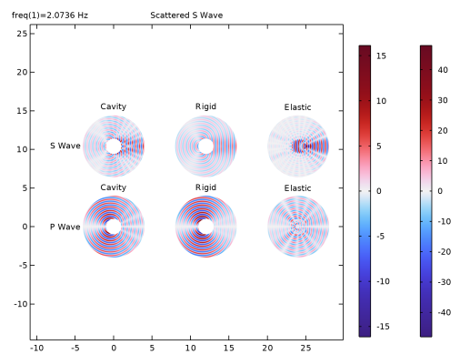
In the Settings window for Surface, click Replace Expression in the upper-right corner of the Expression section. From the menu, choose Component 1 (comp1) > Solid Mechanics > Displacement > Curl of displacement (material and geometry frames) > solid.curlUZ - Curl of displacement, Z-component.
3
In the Scattered S Wave toolbar, click  Plot.
Results
Scattered S Wave
In the Model Builder window, collapse the Results > Scattered S Wave node.
Total Displacement Field Magnitude
1
In the Model Builder window, right-click Scattered Displacement Field Magnitude and choose Duplicate.
Add the incident field to the scattered to obtain the total displacement.
2
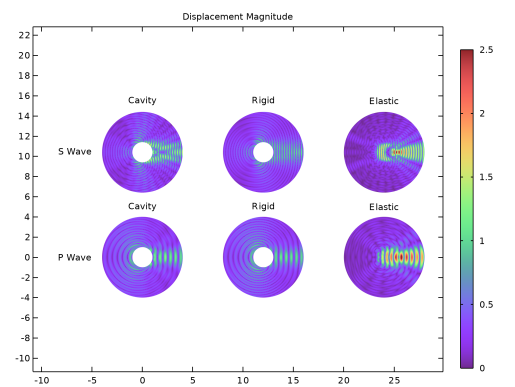
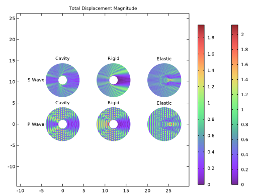
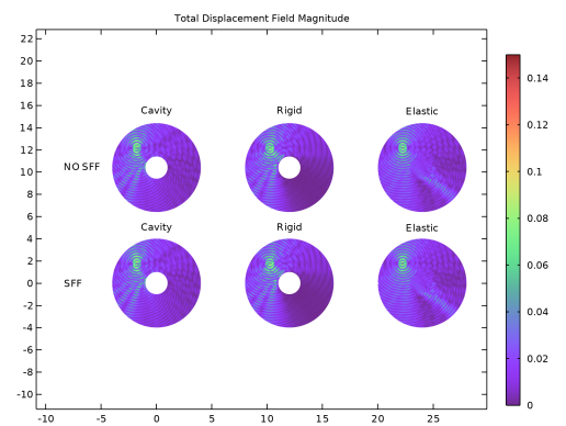
In the Settings window for 2D Plot Group, type Total Displacement Field Magnitude in the Label text field.
3
Locate the Title section. In the Title text area, type Total Displacement Magnitude.
Surface 1
1
In the Model Builder window, expand the Total Displacement Field Magnitude node, then click Surface 1.
2
In the Settings window for Surface, locate the Expression section.
3
In the Expression text field, type sqrt((real(u+uP))^2+(real(v+vP))^2).
4
In the Total Displacement Field Magnitude toolbar, click  Plot.
Results
Total Displacement Field Magnitude
In the Model Builder window, collapse the Results > Total Displacement Field Magnitude node.
Total P Wave
1
In the Model Builder window, right-click Scattered P Wave and choose Duplicate.
2
In the Model Builder window, click Scattered P Wave 1.
3
In the Settings window for 2D Plot Group, type Total P Wave in the Label text field.
Surface 1
1
In the Model Builder window, click Surface 1.
2
In the Settings window for Surface, locate the Expression section.
3
In the Expression text field, type d(u+uP,x)+d(v+vP,y).
Results
Total P Wave
In the Model Builder window, collapse the Results > Total P Wave node.
Total S Wave
1
In the Model Builder window, right-click Scattered S Wave and choose Duplicate.
2
In the Model Builder window, click Scattered S Wave 1.
3
In the Settings window for 2D Plot Group, type Total S Wave in the Label text field.
Surface 1
1
In the Model Builder window, click Surface 1.
2
In the Settings window for Surface, locate the Expression section.
3
In the Expression text field, type d(v+vP,x)-d(u+uP,y).
4
In the Total S Wave toolbar, click  Plot.
Now analyze the case of impinging S wave.
Definitions
Incident S Wave
1
In the Model Builder window, right-click Incident P Wave and choose Duplicate.
2
In the Settings window for Variables, type Incident S Wave in the Label text field.
3
Locate the Variables section. In the table, enter the following settings:
Solid Mechanics (solid)
Body Load (Elastic Inclusion), P Wave, Cavity Inclusion, P Wave, Elastic Inclusion, P Wave, Infinitely Rigid Inclusion, P Wave
1
In the Model Builder window, under Component 1 (comp1) > Solid Mechanics (solid), Ctrl-click to select Cavity Inclusion, P Wave, Infinitely Rigid Inclusion, P Wave, Elastic Inclusion, P Wave, and Body Load (Elastic Inclusion), P Wave.
2
P Wave
In the Settings window for Group, type P Wave in the Label text field.
P Wave 1
Right-click P Wave and choose Duplicate.
P Wave
In the Model Builder window, collapse the Component 1 (comp1) > Solid Mechanics (solid) > P Wave node.
S Wave
1
In the Model Builder window, under Component 1 (comp1) > Solid Mechanics (solid) click P Wave 1.
2
In the Settings window for Group, type S Wave in the Label text field.
Cavity Inclusion, S Wave
1
In the Model Builder window, expand the S Wave node, then click Cavity Inclusion, P Wave 1.
2
In the Settings window for Boundary Load, type Cavity Inclusion, S Wave in the Label text field.
3
Locate the Force section. Specify the fA vector as
Infinitely Rigid Inclusion, S Wave
1
In the Model Builder window, under Component 1 (comp1) > Solid Mechanics (solid) > S Wave click Infinitely Rigid Inclusion, P Wave 1.
2
In the Settings window for Prescribed Displacement, type Infinitely Rigid Inclusion, S Wave in the Label text field.
3
Locate the Prescribed Displacement section. In the u0x text field, type -uS.
4
In the u0y text field, type -vS.
Elastic Inclusion, S Wave
1
In the Model Builder window, expand the Component 1 (comp1) > Solid Mechanics (solid) > S Wave > Elastic Inclusion, P Wave 1 node, then click Elastic Inclusion, P Wave 1.
2
In the Settings window for Linear Elastic Material, type Elastic Inclusion, S Wave in the Label text field.
Initial Stress and Strain
1
In the Model Builder window, under Component 1 (comp1) > Solid Mechanics (solid) > S Wave > Elastic Inclusion, S Wave click Initial Stress and Strain 1.
2
In the Settings window for Initial Stress and Strain, type Initial Stress and Strain in the Label text field.
3
Locate the Initial Stress and Strain section. Specify the S0 matrix as
4
Specify the ε0 matrix as
Body Load (Elastic Inclusion), S Wave
1
In the Model Builder window, under Component 1 (comp1) > Solid Mechanics (solid) > S Wave click Body Load (Elastic Inclusion), P Wave 1.
2
In the Settings window for Body Load, type Body Load (Elastic Inclusion), S Wave in the Label text field.
3
Locate the Force section. Specify the fV vector as
Elastic Inclusion, S Wave
In the Model Builder window, collapse the Component 1 (comp1) > Solid Mechanics (solid) > S Wave > Elastic Inclusion, S Wave node.
Solid Mechanics (solid)
S Wave
In the Model Builder window, collapse the Component 1 (comp1) > Solid Mechanics (solid) > S Wave node.
Modify the previous study to include only the desired boundary conditions for future reruns.
P Wave
Step 1: Frequency Domain
1
In the Model Builder window, under P Wave click Step 1: Frequency Domain.
2
In the Settings window for Frequency Domain, locate the Physics and Variables Selection section.
3
Select the Modify model configuration for study step checkbox.
4
In the tree, select Component 1 (comp1) > Solid Mechanics (solid) > S Wave.
5
Click  Disable.
P Wave
In the Model Builder window, collapse the P Wave node.
Add Study
1
In the Study toolbar, click  Add Study to open the Add Study window.
2
Go to the Add Study window.
3
Find the Studies subsection. In the Select Study tree, select General Studies > Frequency Domain.
4
Click the Add Study button in the window toolbar.
S Wave
1
In the Settings window for Study, type S Wave in the Label text field.
2
Locate the Study Settings section. Clear the Generate default plots checkbox.
1
In the Model Builder window, under S Wave click Step 1: Frequency Domain.
2
In the Settings window for Frequency Domain, locate the Study Settings section.
3
In the Frequencies text field, type omega/2/pi[rad].
4
Locate the Physics and Variables Selection section. Select the Modify model configuration for study step checkbox.
5
In the tree, select Component 1 (comp1) > Solid Mechanics (solid) > P Wave.
6
Click  Disable.
7
In the Study toolbar, click  Compute.
8
In the Study toolbar, click  Add Study to close the Add Study window.
Results
Add the results for the incident S wave near those obtained for the P wave.
Scattered u Field
1
In the Model Builder window, under Results click Scattered u Field.
2
In the Settings window for 2D Plot Group, click to expand the Plot Array section.
3
From the Array type list, choose Linear.
4
From the Array axis list, choose y.
Incident P Wave
1
In the Model Builder window, expand the Scattered u Field node, then click Surface 1.
2
In the Settings window for Surface, type Incident P Wave in the Label text field.
Incident S Wave
1
Right-click Incident P Wave and choose Duplicate.
2
In the Settings window for Surface, type Incident S Wave in the Label text field.
3
Locate the Data section. From the Dataset list, choose S Wave/Solution 2 (sol2).
4
In the Scattered u Field toolbar, click  Plot.
5
Click the  Zoom Extents button in the Graphics toolbar.
Table Annotation 1
1
In the Model Builder window, click Table Annotation 1.
2
In the Settings window for Table Annotation, locate the Data section.
3
Scattered u Field
In the Model Builder window, click Scattered u Field.
Table Annotation 2
1
In the Scattered u Field toolbar, click  More Plots and choose Table Annotation.
2
In the Settings window for Table Annotation, locate the Data section.
3
From the Source list, choose Local table.
4
5
Locate the Coloring and Style section. From the Anchor point list, choose Middle left.
6
Clear the Show point checkbox.
7
In the Scattered u Field toolbar, click  Plot.
8
Click the  Zoom Extents button in the Graphics toolbar.
Incident P Wave
1
In the Model Builder window, click Incident P Wave.
2
In the Settings window for Surface, click to expand the Range section.
3
Select the Manual color range checkbox.
4
In the Minimum text field, type -1.5.
5
In the Maximum text field, type 1.5.
Incident S Wave
1
In the Model Builder window, click Incident S Wave.
2
In the Settings window for Surface, click to expand the Inherit Style section.
3
From the Plot list, choose Incident P Wave.
4
In the Scattered u Field toolbar, click  Plot.
Scattered u Field
1
Click the  Zoom Extents button in the Graphics toolbar.
2
In the Model Builder window, click Scattered u Field.
3
In the Settings window for 2D Plot Group, locate the Plot Settings section.
4
From the View list, choose New view.
5
In the Scattered u Field toolbar, click  Plot.
Scattered v Field
1
In the Model Builder window, click Scattered v Field.
2
In the Settings window for 2D Plot Group, locate the Plot Array section.
3
From the Array type list, choose Linear.
4
From the Array axis list, choose y.
Incident P Wave
1
In the Model Builder window, expand the Scattered v Field node, then click Surface 1.
2
In the Settings window for Surface, type Incident P Wave in the Label text field.
Incident S Wave
1
Right-click Incident P Wave and choose Duplicate.
2
In the Settings window for Surface, type Incident S Wave in the Label text field.
3
Locate the Data section. From the Dataset list, choose S Wave/Solution 2 (sol2).
Incident P Wave
1
In the Model Builder window, click Incident P Wave.
2
In the Settings window for Surface, locate the Range section.
3
Select the Manual color range checkbox.
4
In the Minimum text field, type -1.5.
5
In the Maximum text field, type 1.5.
Incident S Wave
1
In the Model Builder window, click Incident S Wave.
2
In the Settings window for Surface, locate the Inherit Style section.
3
From the Plot list, choose Incident P Wave.
Table Annotation 1
1
In the Model Builder window, click Table Annotation 1.
2
In the Settings window for Table Annotation, locate the Data section.
3
Scattered v Field
In the Model Builder window, click Scattered v Field.
Table Annotation 2
1
In the Scattered v Field toolbar, click  More Plots and choose Table Annotation.
2
In the Settings window for Table Annotation, locate the Data section.
3
From the Source list, choose Local table.
4
5
Locate the Coloring and Style section. From the Anchor point list, choose Middle left.
6
Clear the Show point checkbox.
7
In the Scattered v Field toolbar, click  Plot.
Scattered v Field
1
In the Model Builder window, click Scattered v Field.
2
3
Click the  Zoom Extents button in the Graphics toolbar.
4
In the Settings window for 2D Plot Group, locate the Plot Settings section.
5
From the View list, choose View 2D 2.
Scattered Displacement Field Magnitude
1
In the Model Builder window, click Scattered Displacement Field Magnitude.
2
In the Settings window for 2D Plot Group, locate the Plot Array section.
3
From the Array type list, choose Linear.
4
From the Array axis list, choose y.
Incident P Wave
1
In the Model Builder window, expand the Scattered Displacement Field Magnitude node, then click Surface 1.
2
In the Settings window for Surface, type Incident P Wave in the Label text field.
Incident S Wave
1
Right-click Incident P Wave and choose Duplicate.
2
In the Settings window for Surface, type Incident S Wave in the Label text field.
3
Locate the Data section. From the Dataset list, choose S Wave/Solution 2 (sol2).
Incident P Wave
1
In the Model Builder window, click Incident P Wave.
2
In the Settings window for Surface, locate the Range section.
3
Select the Manual color range checkbox.
4
In the Minimum text field, type 0.
5
In the Maximum text field, type 2.5.
Incident S Wave
1
In the Model Builder window, click Incident S Wave.
2
In the Settings window for Surface, click to collapse the Inherit Style section.
3
Click to expand the Inherit Style section. From the Plot list, choose Incident P Wave.
Table Annotation 1
1
In the Model Builder window, click Table Annotation 1.
2
In the Settings window for Table Annotation, locate the Data section.
3
Scattered Displacement Field Magnitude
In the Model Builder window, click Scattered Displacement Field Magnitude.
Table Annotation 2
1
In the Scattered Displacement Field Magnitude toolbar, click  More Plots and choose Table Annotation.
2
In the Settings window for Table Annotation, locate the Data section.
3
From the Source list, choose Local table.
4
5
Locate the Coloring and Style section. From the Anchor point list, choose Middle left.
6
Clear the Show point checkbox.
7
In the Scattered Displacement Field Magnitude toolbar, click  Plot.
Scattered Displacement Field Magnitude
1
Click the  Zoom Extents button in the Graphics toolbar.
2
In the Model Builder window, click Scattered Displacement Field Magnitude.
3
In the Settings window for 2D Plot Group, locate the Plot Settings section.
4
From the View list, choose View 2D 2.
The resulting plot is shown in Figure 1.
Scattered P Wave
1
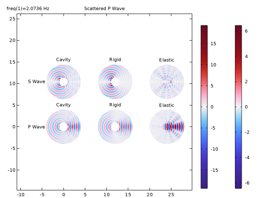
In the Model Builder window, expand the Results > Scattered P Wave node, then click Scattered P Wave.
2
In the Settings window for 2D Plot Group, locate the Plot Array section.
3
From the Array type list, choose Linear.
4
From the Array axis list, choose y.
Incident P Wave
1
In the Model Builder window, under Results > Scattered P Wave click Surface 1.
2
In the Settings window for Surface, type Incident P Wave in the Label text field.
Incident S Wave
1
Right-click Incident P Wave and choose Duplicate.
2
In the Settings window for Surface, type Incident S Wave in the Label text field.
3
Locate the Data section. From the Dataset list, choose S Wave/Solution 2 (sol2).
Table Annotation 1
1
In the Model Builder window, click Table Annotation 1.
2
In the Settings window for Table Annotation, locate the Data section.
3
Scattered P Wave
In the Model Builder window, click Scattered P Wave.
Table Annotation 2
1
In the Scattered P Wave toolbar, click  More Plots and choose Table Annotation.
2
In the Settings window for Table Annotation, locate the Data section.
3
From the Source list, choose Local table.
4
5
Locate the Coloring and Style section. From the Anchor point list, choose Middle left.
6
Clear the Show point checkbox.
7
In the Scattered P Wave toolbar, click  Plot.
Scattered P Wave
1
Click the  Zoom Extents button in the Graphics toolbar.
2
In the Model Builder window, click Scattered P Wave.
3
In the Settings window for 2D Plot Group, locate the Plot Settings section.
4
From the View list, choose View 2D 2.
The resulting plot is shown in Figure 2.
Scattered S Wave
1
In the Model Builder window, click Scattered S Wave.
2
In the Settings window for 2D Plot Group, locate the Plot Array section.
3
From the Array type list, choose Linear.
4
From the Array axis list, choose y.
Incident P Wave
1
In the Model Builder window, expand the Scattered S Wave node, then click Surface 1.
2
In the Settings window for Surface, type Incident P Wave in the Label text field.
Incident S Wave
1
Right-click Incident P Wave and choose Duplicate.
2
In the Settings window for Surface, type Incident S Wave in the Label text field.
3
Locate the Data section. From the Dataset list, choose S Wave/Solution 2 (sol2).
4
In the Scattered S Wave toolbar, click  Plot.
Table Annotation 1
1
In the Model Builder window, click Table Annotation 1.
2
In the Settings window for Table Annotation, locate the Data section.
3
Scattered S Wave
In the Model Builder window, click Scattered S Wave.
Table Annotation 2
1
In the Scattered S Wave toolbar, click  More Plots and choose Table Annotation.
2
In the Settings window for Table Annotation, locate the Data section.
3
From the Source list, choose Local table.
4
5
Locate the Coloring and Style section. From the Anchor point list, choose Middle left.
6
Clear the Show point checkbox.
7
In the Scattered S Wave toolbar, click  Plot.
Scattered S Wave
1
Click the  Zoom Extents button in the Graphics toolbar.
2
In the Model Builder window, click Scattered S Wave.
3
In the Settings window for 2D Plot Group, locate the Plot Settings section.
4
From the View list, choose View 2D 2.
The resulting plot is shown in Figure 3.
Total Displacement Field Magnitude
1
In the Model Builder window, expand the Results > Total Displacement Field Magnitude node, then click Total Displacement Field Magnitude.
2
In the Settings window for 2D Plot Group, locate the Plot Array section.
3
From the Array type list, choose Linear.
4
From the Array axis list, choose y.
Incident P Wave
1
In the Model Builder window, under Results > Total Displacement Field Magnitude click Surface 1.
2
In the Settings window for Surface, type Incident P Wave in the Label text field.
Incident S Wave
1
Right-click Incident P Wave and choose Duplicate.
2
In the Settings window for Surface, type Incident S Wave in the Label text field.
3
Locate the Data section. From the Dataset list, choose S Wave/Solution 2 (sol2).
4
Locate the Expression section. In the Expression text field, type sqrt((real(u+uS))^2+(real(v+vS))^2).
Table Annotation 1
1
In the Model Builder window, click Table Annotation 1.
2
In the Settings window for Table Annotation, locate the Data section.
3
Total Displacement Field Magnitude
In the Model Builder window, click Total Displacement Field Magnitude.
Table Annotation 2
1
In the Total Displacement Field Magnitude toolbar, click  More Plots and choose Table Annotation.
2
In the Settings window for Table Annotation, locate the Data section.
3
From the Source list, choose Local table.
4
5
Locate the Coloring and Style section. From the Anchor point list, choose Middle left.
6
Clear the Show point checkbox.
7
In the Total Displacement Field Magnitude toolbar, click  Plot.
Total Displacement Field Magnitude
1
Click the  Zoom Extents button in the Graphics toolbar.
2
In the Model Builder window, click Total Displacement Field Magnitude.
3
In the Settings window for 2D Plot Group, locate the Plot Settings section.
4
From the View list, choose View 2D 2.
The resulting plot is shown in Figure 4.
Total P Wave
1
In the Model Builder window, expand the Results > Total P Wave node, then click Total P Wave.
2
In the Settings window for 2D Plot Group, locate the Plot Array section.
3
From the Array type list, choose Linear.
4
From the Array axis list, choose y.
Incident P Wave
1
In the Model Builder window, under Results > Total P Wave click Surface 1.
2
In the Settings window for Surface, type Incident P Wave in the Label text field.
Incident S Wave
1
Right-click Incident P Wave and choose Duplicate.
2
In the Settings window for Surface, type Incident S Wave in the Label text field.
3
Locate the Data section. From the Dataset list, choose S Wave/Solution 2 (sol2).
4
Locate the Expression section. In the Expression text field, type d(u+uS,x)+d(v+vS,y).
5
In the Total P Wave toolbar, click  Plot.
Table Annotation 1
1
In the Model Builder window, click Table Annotation 1.
2
In the Settings window for Table Annotation, locate the Data section.
3
Total P Wave
In the Model Builder window, click Total P Wave.
Table Annotation 2
1
In the Total P Wave toolbar, click  More Plots and choose Table Annotation.
2
In the Settings window for Table Annotation, locate the Data section.
3
From the Source list, choose Local table.
4
5
Locate the Coloring and Style section. From the Anchor point list, choose Middle left.
6
Clear the Show point checkbox.
7
In the Total P Wave toolbar, click  Plot.
Total P Wave
1
Click the  Zoom Extents button in the Graphics toolbar.
2
In the Model Builder window, click Total P Wave.
3
In the Settings window for 2D Plot Group, locate the Plot Settings section.
4
From the View list, choose View 2D 2.
The resulting plot is shown in Figure 5.
Total S Wave
1
In the Model Builder window, click Total S Wave.
2
In the Settings window for 2D Plot Group, locate the Plot Array section.
3
From the Array type list, choose Linear.
4
From the Array axis list, choose y.
Incident P Wave
1
In the Model Builder window, under Results > Total S Wave click Surface 1.
2
In the Settings window for Surface, type Incident P Wave in the Label text field.
Incident S Wave
1
Right-click Incident P Wave and choose Duplicate.
2
In the Settings window for Surface, type Incident S Wave in the Label text field.
3
Locate the Data section. From the Dataset list, choose S Wave/Solution 2 (sol2).
4
Locate the Expression section. In the Expression text field, type d(v+vS,x)-d(u+uS,y).
Table Annotation 1
1
In the Model Builder window, click Table Annotation 1.
2
In the Settings window for Table Annotation, locate the Data section.
3
Total S Wave
In the Model Builder window, click Total S Wave.
Table Annotation 2
1
In the Total S Wave toolbar, click  More Plots and choose Table Annotation.
2
In the Settings window for Table Annotation, locate the Data section.
3
From the Source list, choose Local table.
4
5
Locate the Coloring and Style section. From the Anchor point list, choose Middle left.
6
Clear the Show point checkbox.
7
In the Total S Wave toolbar, click  Plot.
Total S Wave
1
Click the  Zoom Extents button in the Graphics toolbar.
2
In the Model Builder window, click Total S Wave.
3
In the Settings window for 2D Plot Group, locate the Plot Settings section.
4
From the View list, choose View 2D 2.
The resulting plot is shown in Figure 6.
5
In the Model Builder window, collapse the Total S Wave node.
Total P Wave
In the Model Builder window, collapse the Results > Total P Wave node.
Total Displacement Field Magnitude
In the Model Builder window, collapse the Results > Total Displacement Field Magnitude node.
Scattered S Wave
In the Model Builder window, collapse the Results > Scattered S Wave node.
Scattered P Wave
In the Model Builder window, collapse the Results > Scattered P Wave node.
Scattered Displacement Field Magnitude
In the Model Builder window, collapse the Results > Scattered Displacement Field Magnitude node.
Scattered v Field
In the Model Builder window, collapse the Results > Scattered v Field node.
Scattered u Field
In the Model Builder window, collapse the Results > Scattered u Field node.
Scattered Displacement Field Magnitude, Scattered P Wave, Scattered S Wave, Scattered u Field, Scattered v Field, Total Displacement Field Magnitude, Total P Wave, Total S Wave
1
In the Model Builder window, under Results, Ctrl-click to select Scattered u Field, Scattered v Field, Scattered Displacement Field Magnitude, Scattered P Wave, Scattered S Wave, Total Displacement Field Magnitude, Total P Wave, and Total S Wave.
2
Plane Wave
In the Settings window for Group, type Plane Wave in the Label text field.
Add a point where to apply the point source.
Geometry 1
Point 1 (pt1)
1
In the Geometry toolbar, click  Point.
2
In the Settings window for Point, locate the Point section.
3
In the x text field, type -((R-r_layer-r_o)/2+r_o)*cos(pi/4).
4
In the y text field, type ((R-r_layer-r_o)/2+r_o)*sin(pi/4).
5
Click  Build Selected.
6
Drag and drop below Circle 1 (c1).
7
Click  Build Selected.
Array 1 (arr1)
1
In the Model Builder window, click Array 1 (arr1).
2
Click the  Select All button in the Graphics toolbar.
3
In the Settings window for Array, click  Build All Objects.
Solid Mechanics (solid)
Point Load 1
1
In the Physics toolbar, click  Points and choose Point Load.
2
3
In the Settings window for Point Load, locate the Force section.
4
Specify the FP vector as
Add Study
1
In the Home toolbar, click  Add Study to open the Add Study window.
2
Go to the Add Study window.
3
Find the Studies subsection. In the Select Study tree, select General Studies > Frequency Domain.
4
Click the Add Study button in the window toolbar.
5
In the Home toolbar, click  Add Study to close the Add Study window.
Point Source Incident Field
1
In the Settings window for Study, locate the Study Settings section.
2
Clear the Generate default plots checkbox.
3
In the Label text field, type Point Source Incident Field.
P Wave
Step 1: Frequency Domain
1
In the Model Builder window, expand the P Wave node, then click Step 1: Frequency Domain.
2
In the Settings window for Frequency Domain, locate the Physics and Variables Selection section.
3
In the tree, select Component 1 (comp1) > Solid Mechanics (solid) > Point Load 1.
4
Click  Disable.
P Wave
In the Model Builder window, collapse the P Wave node.
S Wave
1
In the Model Builder window, under S Wave click Step 1: Frequency Domain.
2
In the Settings window for Frequency Domain, locate the Physics and Variables Selection section.
3
Click  Disable.
S Wave
In the Model Builder window, collapse the S Wave node.
Point Source Incident Field
1
In the Model Builder window, under Point Source Incident Field click Step 1: Frequency Domain.
2
In the Settings window for Frequency Domain, locate the Study Settings section.
3
In the Frequencies text field, type omega/2/pi[rad].
4
Locate the Physics and Variables Selection section. Select the Modify model configuration for study step checkbox.
5
In the tree, select Component 1 (comp1) > Solid Mechanics (solid) > P Wave.
6
Click  Disable.
7
In the tree, select Component 1 (comp1) > Solid Mechanics (solid) > S Wave.
8
Click  Disable.
9
In the Study toolbar, click  Compute.
Plot the field generated by the point source, that will be used as incident field.
Results
Point Source Background Fields
1
In the Results toolbar, click  2D Plot Group.
2
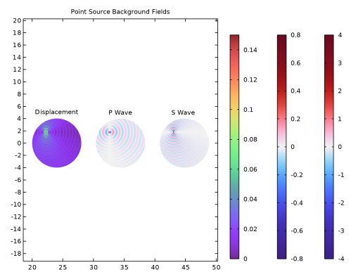
In the Settings window for 2D Plot Group, type Point Source Background Fields in the Label text field.
3
Locate the Data section. From the Dataset list, choose Point Source Incident Field/Solution 3 (sol3).
4
Locate the Plot Settings section. Clear the Plot dataset edges checkbox.
5
Locate the Plot Array section. From the Array type list, choose Linear.
Displacement Magnitude
1
Right-click Point Source Background Fields and choose Surface.
2
In the Settings window for Surface, type Displacement Magnitude in the Label text field.
3
Locate the Coloring and Style section. From the Color table list, choose SpectrumLight.
Selection 1
1
Right-click Displacement Magnitude and choose Selection.
2
3
In the Point Source Background Fields toolbar, click  Plot.
Displacement Magnitude
1
In the Model Builder window, click Displacement Magnitude.
2
In the Settings window for Surface, locate the Range section.
3
Select the Manual color range checkbox.
4
In the Minimum text field, type 0.
5
In the Maximum text field, type 0.15.
6
In the Point Source Background Fields toolbar, click  Plot.
P Wave
1
Right-click Displacement Magnitude and choose Duplicate.
2
In the Settings window for Surface, type P Wave in the Label text field.
3
Locate the Expression section. In the Expression text field, type d(u,x)+d(v,y).
4
Locate the Range section. Clear the Manual color range checkbox.
5
Locate the Coloring and Style section. From the Color table list, choose Wave.
6
Locate the Range section. Select the Manual color range checkbox.
7
In the Minimum text field, type -0.8.
8
In the Maximum text field, type 0.8.
9
In the Point Source Background Fields toolbar, click  Plot.
P Wave 1
Right-click P Wave and choose Duplicate.
S Wave
1
In the Model Builder window, expand the Results > Point Source Background Fields > P Wave node, then click Results > Point Source Background Fields > P Wave 1.
2
In the Settings window for Surface, type S Wave in the Label text field.
3
Locate the Expression section. In the Expression text field, type d(v,x)-d(u,y).
4
In the Point Source Background Fields toolbar, click  Plot.
5
Click the  Zoom Extents button in the Graphics toolbar.
6
Locate the Range section. In the Minimum text field, type -4.
7
In the Maximum text field, type 4.
8
In the Point Source Background Fields toolbar, click  Plot.
9
Click the  Zoom Extents button in the Graphics toolbar.
Point Source Background Fields
In the Model Builder window, click Point Source Background Fields.
Table Annotation 1
1
In the Point Source Background Fields toolbar, click  More Plots and choose Table Annotation.
2
In the Settings window for Table Annotation, locate the Data section.
3
From the Source list, choose Local table.
4
5
Locate the Coloring and Style section. Clear the Show point checkbox.
6
From the Anchor point list, choose Center.
7
In the Point Source Background Fields toolbar, click  Plot.
The resulting plot is shown in Figure 7.
Point Source Background Fields
1
In the Model Builder window, click Point Source Background Fields.
2
In the Settings window for 2D Plot Group, locate the Title section.
3
From the Title type list, choose Manual.
4
In the Title text area, type Point Source Background Fields.
5
Clear the Parameter indicator text field.
6
Click the  Zoom Extents button in the Graphics toolbar.
View 2D 3
In the Model Builder window, under Results right-click Views and choose View 2D.
Point Source Background Fields
1
In the Settings window for 2D Plot Group, locate the Plot Settings section.
2
From the View list, choose View 2D 3.
P Wave
In the Model Builder window, collapse the Results > Point Source Background Fields > P Wave node.
Displacement Magnitude
In the Model Builder window, collapse the Results > Point Source Background Fields > Displacement Magnitude node.
Point Source Background Fields
In the Model Builder window, collapse the Results > Point Source Background Fields node.
Set the results of the previous study to be the new incident field.
Definitions
Point Source
1
In the Model Builder window, right-click Incident S Wave and choose Duplicate.
2
In the Settings window for Variables, type Point Source in the Label text field.
3
Locate the Variables section. In the table, enter the following settings:
Note that the point source background field is only defined on the third computational domain. Add two General Extrusion operators in order to make the point source background field available also for the other two computational domains.
General Extrusion 1 (genext1)
1
In the Definitions toolbar, click  Nonlocal Couplings and choose General Extrusion.
2
3
In the Settings window for General Extrusion, locate the Destination Map section.
4
In the x-expression text field, type x+24.
General Extrusion 2 (genext2)
1
Right-click General Extrusion 1 (genext1) and choose Duplicate.
2
In the Settings window for General Extrusion, locate the Destination Map section.
3
In the x-expression text field, type x+12.
Solid Mechanics (solid)
Point Source
1
In the Model Builder window, expand the Component 1 (comp1) > Solid Mechanics (solid) > P Wave > Cavity Inclusion, P Wave node.
2
Right-click S Wave and choose Duplicate.
3
In the Settings window for Group, type Point Source in the Label text field.
Cavity Inclusion, Point Source
1
In the Model Builder window, expand the Point Source node, then click Cavity Inclusion, S Wave 1.
2
In the Settings window for Boundary Load, type Cavity Inclusion, Point Source in the Label text field.
3
Locate the Force section. Specify the fA vector as
Infinitely Rigid Inclusion, Point Source
1
In the Model Builder window, under Component 1 (comp1) > Solid Mechanics (solid) > Point Source click Infinitely Rigid Inclusion, S Wave 1.
2
In the Settings window for Prescribed Displacement, type Infinitely Rigid Inclusion, Point Source in the Label text field.
3
Locate the Prescribed Displacement section. In the u0x text field, type -genext2(uPS).
4
In the u0y text field, type -genext2(vPS).
Elastic Inclusion, Point Source
1
In the Model Builder window, expand the Component 1 (comp1) > Solid Mechanics (solid) > Point Source > Elastic Inclusion, S Wave 1 node, then click Elastic Inclusion, S Wave 1.
2
In the Settings window for Linear Elastic Material, type Elastic Inclusion, Point Source in the Label text field.
Initial Stress and Strain
1
In the Model Builder window, click Initial Stress and Strain.
2
In the Settings window for Initial Stress and Strain, locate the Initial Stress and Strain section.
3
Specify the S0 matrix as
4
Specify the ε0 matrix as
Body load (Elastic Inclusion), Point Source
1
In the Model Builder window, under Component 1 (comp1) > Solid Mechanics (solid) > Point Source click Body Load (Elastic Inclusion), S Wave 1.
2
In the Settings window for Body Load, type Body load (Elastic Inclusion), Point Source in the Label text field.
3
Locate the Force section. Specify the fV vector as
Elastic Inclusion, Point Source
In the Model Builder window, collapse the Component 1 (comp1) > Solid Mechanics (solid) > Point Source > Elastic Inclusion, Point Source node.
Solid Mechanics (solid)
Point Source
In the Model Builder window, collapse the Component 1 (comp1) > Solid Mechanics (solid) > Point Source node.
Add Study
1
In the Home toolbar, click  Add Study to open the Add Study window.
2
Go to the Add Study window.
3
Find the Studies subsection. In the Select Study tree, select General Studies > Frequency Domain.
4
Click the Add Study button in the window toolbar.
5
In the Home toolbar, click  Add Study to close the Add Study window.
Point Source Scattered Field
1
In the Settings window for Study, type Point Source Scattered Field in the Label text field.
2
Locate the Study Settings section. Clear the Generate default plots checkbox.
P Wave
Step 1: Frequency Domain
1
In the Model Builder window, expand the P Wave node, then click Step 1: Frequency Domain.
2
In the Settings window for Frequency Domain, locate the Physics and Variables Selection section.
3
In the tree, select Component 1 (comp1) > Solid Mechanics (solid) > Point Source.
4
Click  Disable.
S Wave
1
In the Model Builder window, expand the S Wave node, then click Step 1: Frequency Domain.
2
In the Settings window for Frequency Domain, locate the Physics and Variables Selection section.
3
In the tree, select Component 1 (comp1) > Solid Mechanics (solid) > Point Source.
4
Click  Disable.
Point Source Incident Field
1
In the Model Builder window, under Point Source Incident Field click Step 1: Frequency Domain.
2
In the Settings window for Frequency Domain, locate the Physics and Variables Selection section.
3
In the tree, select Component 1 (comp1) > Solid Mechanics (solid) > Point Source.
4
Click  Disable.
Point Source Scattered Field
1
In the Model Builder window, under Point Source Scattered Field click Step 1: Frequency Domain.
2
In the Settings window for Frequency Domain, locate the Study Settings section.
3
In the Frequencies text field, type omega/2/pi[rad].
4
Locate the Physics and Variables Selection section. Select the Modify model configuration for study step checkbox.
5
In the tree, select Component 1 (comp1) > Solid Mechanics (solid) > P Wave.
6
Click  Disable.
7
In the tree, select Component 1 (comp1) > Solid Mechanics (solid) > S Wave.
8
Click  Disable.
9
In the tree, select Component 1 (comp1) > Solid Mechanics (solid) > Point Load 1.
10
Click  Disable.
11
In the Study toolbar, click  Compute.
Results
Point Source Scattered Displacement Field Magnitude
1
In the Results toolbar, click  2D Plot Group.
2
In the Settings window for 2D Plot Group, type Point Source Scattered Displacement Field Magnitude in the Label text field.
3
Locate the Title section. From the Title type list, choose Manual.
4
In the Title text area, type Displacement Magnitude.
5
Clear the Parameter indicator text field.
6
Locate the Data section. From the Dataset list, choose Point Source Scattered Field/Solution 4 (sol4).
Surface 1
Right-click Point Source Scattered Displacement Field Magnitude and choose Surface.
Selection 1
1
In the Model Builder window, right-click Surface 1 and choose Selection.
2
Surface 1
1
In the Model Builder window, click Surface 1.
2
In the Settings window for Surface, locate the Coloring and Style section.
3
From the Color table list, choose SpectrumLight.
Point Source Scattered Displacement Field Magnitude
1
In the Model Builder window, click Point Source Scattered Displacement Field Magnitude.
2
In the Settings window for 2D Plot Group, locate the Plot Settings section.
3
Clear the Plot dataset edges checkbox.
Table Annotation 1
1
In the Point Source Scattered Displacement Field Magnitude toolbar, click  More Plots and choose Table Annotation.
2
In the Settings window for Table Annotation, locate the Data section.
3
From the Source list, choose Local table.
4
5
Locate the Coloring and Style section. Clear the Show point checkbox.
6
From the Anchor point list, choose Center.
The resulting plot is shown in Figure 8.
View 2D 4
In the Model Builder window, under Results right-click Views and choose View 2D.
Point Source Scattered Displacement Field Magnitude
1
In the Settings window for 2D Plot Group, locate the Plot Settings section.
2
From the View list, choose View 2D 4.
3
Click the  Zoom Extents button in the Graphics toolbar.
Surface 1
In the Model Builder window, collapse the Results > Point Source Scattered Displacement Field Magnitude > Surface 1 node.
Point Source Scattered Displacement Field Magnitude 1
Right-click Results > Point Source Scattered Displacement Field Magnitude and choose Duplicate.
Point Source Scattered Displacement Field Magnitude
In the Model Builder window, collapse the Results > Point Source Scattered Displacement Field Magnitude node.
Point Source Total Displacement Field Magnitude
1
In the Model Builder window, under Results click Point Source Scattered Displacement Field Magnitude 1.
2
In the Settings window for 2D Plot Group, type Point Source Total Displacement Field Magnitude in the Label text field.
3
In the Model Builder window, expand the Point Source Total Displacement Field Magnitude node.
Scattered Field Formulation
1
In the Model Builder window, expand the Results > Point Source Total Displacement Field Magnitude > Surface 1 node, then click Surface 1.
2
In the Settings window for Surface, type Scattered Field Formulation in the Label text field.
3
Locate the Expression section. In the Expression text field, type if(x>20,sqrt((real(u+uPS))^2+(real(v+vPS))^2),if(x<5,sqrt((real(u+genext1(uPS)))^2+(real(v+genext1(vPS)))^2),sqrt((real(u+genext2(uPS)))^2+(real(v+genext2(vPS)))^2))).
4
Locate the Range section. Select the Manual color range checkbox.
5
In the Minimum text field, type 0.
6
In the Maximum text field, type 0.15.
7
In the Point Source Total Displacement Field Magnitude toolbar, click  Plot.
Results
Point Source Total Displacement Field Magnitude
1
In the Model Builder window, collapse the Results > Point Source Total Displacement Field Magnitude node.
2
In the Model Builder window, click Point Source Total Displacement Field Magnitude.
3
In the Settings window for 2D Plot Group, locate the Title section.
4
In the Title text area, type Total Displacement Field Magnitude.
Compute the total field without using the scattered field formulation, that is, adopting the actual boundary conditions and field equation for the total field.
Solid Mechanics (solid)
Point Load 1
1
In the Model Builder window, under Component 1 (comp1) > Solid Mechanics (solid) click Point Load 1.
2
Fixed Constraint 1
1
In the Physics toolbar, click  Boundaries and choose Fixed Constraint.
2
Add Study
1
In the Home toolbar, click  Add Study to open the Add Study window.
2
Go to the Add Study window.
3
Find the Studies subsection. In the Select Study tree, select General Studies > Frequency Domain.
4
Click the Add Study button in the window toolbar.
Point Source Total Field (NO Scattered Field Formulation)
1
In the Settings window for Study, type Point Source Total Field (NO Scattered Field Formulation) in the Label text field.
2
Locate the Study Settings section. Clear the Generate default plots checkbox.
P Wave
Step 1: Frequency Domain
1
In the Model Builder window, under P Wave click Step 1: Frequency Domain.
2
In the Settings window for Frequency Domain, locate the Physics and Variables Selection section.
3
In the tree, select Component 1 (comp1) > Solid Mechanics (solid) > Fixed Constraint 1.
4
Click  Disable.
S Wave
1
In the Model Builder window, under S Wave click Step 1: Frequency Domain.
2
In the Settings window for Frequency Domain, locate the Physics and Variables Selection section.
3
In the tree, select Component 1 (comp1) > Solid Mechanics (solid) > Fixed Constraint 1.
4
Click  Disable.
Point Source Incident Field
1
In the Model Builder window, under Point Source Incident Field click Step 1: Frequency Domain.
2
In the Settings window for Frequency Domain, locate the Physics and Variables Selection section.
3
In the tree, select Component 1 (comp1) > Solid Mechanics (solid) > Fixed Constraint 1.
4
Click  Disable.
Point Source Scattered Field
1
In the Model Builder window, under Point Source Scattered Field click Step 1: Frequency Domain.
2
In the Settings window for Frequency Domain, locate the Physics and Variables Selection section.
3
Click  Disable.
Point Source Total Field (NO Scattered Field Formulation)
1
In the Model Builder window, under Point Source Total Field (NO Scattered Field Formulation) click Step 1: Frequency Domain.
2
In the Settings window for Frequency Domain, locate the Study Settings section.
3
In the Frequencies text field, type omega/2/pi[rad].
4
Locate the Physics and Variables Selection section. Select the Modify model configuration for study step checkbox.
5
In the tree, select Component 1 (comp1) > Solid Mechanics (solid) > P Wave.
6
Click  Disable.
7
In the tree, select Component 1 (comp1) > Solid Mechanics (solid) > S Wave.
8
Click  Disable.
9
In the tree, select Component 1 (comp1) > Solid Mechanics (solid) > Point Source > Cavity Inclusion, Point Source.
10
Click  Disable.
11
In the tree, select Component 1 (comp1) > Solid Mechanics (solid) > Point Source > Infinitely Rigid Inclusion, Point Source.
12
Click  Disable.
13
In the tree, select Component 1 (comp1) > Solid Mechanics (solid) > Point Source > Elastic Inclusion, Point Source > Initial Stress and Strain.
14
Click  Disable.
15
In the tree, select Component 1 (comp1) > Solid Mechanics (solid) > Point Source > Body load (Elastic Inclusion), Point Source.
16
Click  Disable.
17
In the Study toolbar, click  Compute.
18
In the Study toolbar, click  Add Study to close the Add Study window.
19
In the Model Builder window, collapse the Point Source Total Field (NO Scattered Field Formulation) node.
Plot the results obtained next to those obtained with the scattered field formulation for comparison.
Results
Point Source Total Displacement Field Magnitude
1
In the Model Builder window, under Results click Point Source Total Displacement Field Magnitude.
2
In the Settings window for 2D Plot Group, locate the Plot Array section.
3
From the Array type list, choose Linear.
4
From the Array axis list, choose y.
NO Scattered Field Formulation
1
In the Model Builder window, expand the Point Source Total Displacement Field Magnitude node.
2
Right-click Scattered Field Formulation and choose Duplicate.
3
In the Settings window for Surface, locate the Data section.
4
From the Dataset list, choose Point Source Total Field (NO Scattered Field Formulation)/Solution 5 (sol5).
5
Locate the Expression section. In the Expression text field, type solid.disp.
6
In the Point Source Total Displacement Field Magnitude toolbar, click  Plot.
7
Locate the Inherit Style section. From the Plot list, choose Scattered Field Formulation.
8
In the Label text field, type NO Scattered Field Formulation.
Table Annotation 1
1
In the Model Builder window, click Table Annotation 1.
2
In the Settings window for Table Annotation, locate the Data section.
3
Point Source Total Displacement Field Magnitude
In the Model Builder window, click Point Source Total Displacement Field Magnitude.
Table Annotation 2
1
In the Point Source Total Displacement Field Magnitude toolbar, click  More Plots and choose Table Annotation.
2
In the Settings window for Table Annotation, locate the Data section.
3
From the Source list, choose Local table.
4
5
Locate the Coloring and Style section. From the Anchor point list, choose Middle left.
6
Clear the Show point checkbox.
7
In the Point Source Total Displacement Field Magnitude toolbar, click  Plot.
8
Click the  Zoom Extents button in the Graphics toolbar.
Point Source Total Displacement Field Magnitude
1
In the Model Builder window, click Point Source Total Displacement Field Magnitude.
2
In the Settings window for 2D Plot Group, locate the Plot Settings section.
3
From the View list, choose New view.
4
In the Point Source Total Displacement Field Magnitude toolbar, click  Plot.
The resulting plot is shown in Figure 9.
Point Source Total P Wave
1
Right-click Point Source Total Displacement Field Magnitude and choose Duplicate.
2
In the Model Builder window, click Point Source Total Displacement Field Magnitude 1.
3
In the Settings window for 2D Plot Group, type Point Source Total P Wave in the Label text field.
Scattered Field Formulation
1
In the Model Builder window, click Scattered Field Formulation.
2
In the Settings window for Surface, locate the Expression section.
3
In the Expression text field, type if(x>20,d(u+uPS,x)+d(v+vPS,y),if(x<5,d(u+genext1(uPS),x)+d(v+genext1(vPS),y),d(u+genext2(uPS),x)+d(v+genext2(vPS),y))).
4
In the Point Source Total P Wave toolbar, click  Plot.
5
Locate the Coloring and Style section. From the Color table list, choose Wave.
6
Locate the Range section. In the Minimum text field, type -0.5.
7
In the Maximum text field, type 0.5.
8
In the Point Source Total P Wave toolbar, click  Plot.
NO Scattered Field Formulation
1
In the Model Builder window, click NO Scattered Field Formulation.
2
In the Settings window for Surface, locate the Expression section.
3
In the Expression text field, type d(u,x)+d(v,y).
4
In the Point Source Total P Wave toolbar, click  Plot.
Point Source Total S Wave
1
In the Model Builder window, right-click Point Source Total P Wave and choose Duplicate.
2
In the Model Builder window, click Point Source Total P Wave 1.
3
In the Settings window for 2D Plot Group, type Point Source Total S Wave in the Label text field.
Scattered Field Formulation
1
In the Model Builder window, click Scattered Field Formulation.
2
In the Settings window for Surface, locate the Expression section.
3
In the Expression text field, type if(x>20,-d(u+uPS,y)+d(v+vPS,x),if(x<5,-d(u+genext1(uPS),y)+d(v+genext1(vPS),x),-d(u+genext2(uPS),y)+d(v+genext2(vPS),x))).
4
Locate the Range section. In the Minimum text field, type -1.
5
In the Maximum text field, type 1.
6
In the Point Source Total S Wave toolbar, click  Plot.
NO Scattered Field Formulation
1
In the Model Builder window, click NO Scattered Field Formulation.
2
In the Settings window for Surface, locate the Expression section.
3
In the Expression text field, type -d(u,y)+d(v,x).
4
In the Point Source Total S Wave toolbar, click  Plot.