PDF

MEMS Microphone with Slip Wall
Introduction
The development in the area of MEMS devices and microphones is fast, and MEMS microphones are becoming a standard part of various products from laptops to earbuds. This tutorial demonstrates how to set up a model of a MEMS microphone consisting of a micro-perforated plate (MPP) and a vibrating membrane, see Figure 1. The design with an MPP and a diaphragm is used in Ref. 1, the geometry in this model is inspired by Ref. 1 but is simplified and uses different parameters.
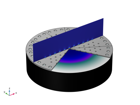
Figure 1: MEMS microphone consisting of a micro-perforated plate (MPP) and a vibrating membrane. The harmonic displacement of the membrane is shown together with the acoustic velocity through the MPP.
The development in manufacturing processes allows to make MEMS devices with smaller length scales. The small length scales lead to high Knudsen numbers and therefore a domain where noncontinuum effects can become important. This model shows how to include a slip velocity boundary condition and thereby increase the range of Knudsen numbers where the finite element model is valid. The slip velocity boundary condition is typically used for Knudsen numbers in the range from 0.001 to 0.01.
Note, the perforation ratio of the MPP in the model is quite low, this is to reduce the number of holes and thus the size of the numerical model.
Model Definition
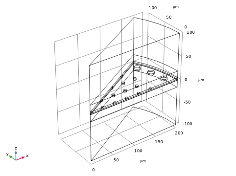
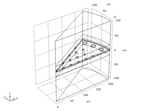
The MEMS microphone consists of an MPP and a vibrating diaphragm, and a closed backing volume. The MEMS microphone is cylindrical with the holes in the MPP placed in a hexagonal lattice structure. The symmetry allows for modeling a 30-degree section of the cylinder.
Figure 2: Geometry of the MEMS microphone. A 30-degree section is modeled with symmetry planes.
The MPP consists of holes with 3 µm radius in a hexagonal structure and vent holes with 7 µm radius at the edge of the plate. The MPP has a thickness of 3 µm, and the diaphragm a thickness of 0.5 µm. The distance between the MPP and diaphragm is 2 µm. Below the diaphragm is a closed backing volume modeled with Thermoviscous Acoustics, and the domain above the MPP; the holes in the MPP; and the gap between the MPP and diaphragm are modeled with Thermoviscous Acoustics.
The Slip Wall boundary condition is applied to the surface of the diaphragm and MPP in the Thermoviscous Acoustics domain. When setting a Slip Wall boundary condition the tangential velocity at the wall will depend on the stress in the fluid at the boundary, thus creating a discontinuity between the velocity of the solid and the fluid.
The diaphragm is prestressed by an electric field which gives a stationary deformation of the diaphragm. The diaphragm is connected to ground while a Terminal on the MPP is connected to an Electrical Circuit. The Electrical Circuit consists of a Resistor and a Voltage Source of 1V. This results in an electric field between the MPP and diaphragm and a deformation which is modeled with Moving Mesh.
In the frequency domain study, a pressure is applied on the surface above the MPP in the Thermoviscous Acoustics domain. The diaphragm will vibrate due to the pressure field, and this will cause a varying electrical signal due to the variations in the distance between the MPP and diaphragm.
To model the correct electric response of the MEMS microphone it is important to model the correct damping in the flow through the holes in the MPP and in the squeezing flow between the MPP and the diaphragm. For small length scales it can be necessary to include the noncontinuum effects with the Slip Wall boundary condition.
Results and Discussion
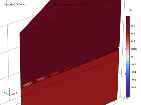
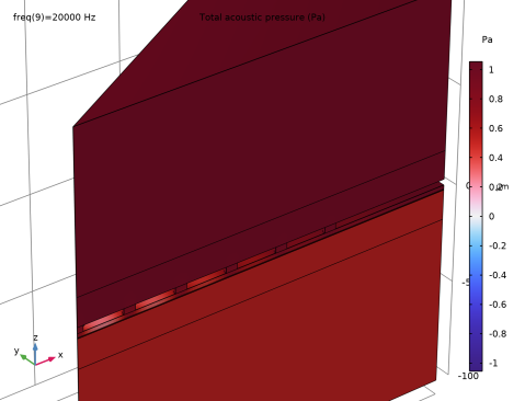
The resulting acoustic pressure in all domains is shown in Figure 3.
Figure 3: Acoustic pressure at 20 kHz.
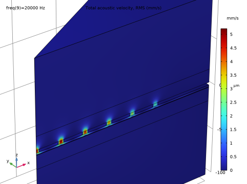
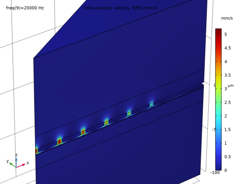
The acoustic velocity is shown in Figure 4. Note the high velocities both through the holes in the MPP and in the squeezing flow between the MPP and the diaphragm. These areas are the sources for the viscous damping in the system.
.
Figure 4: Acoustic pressure.
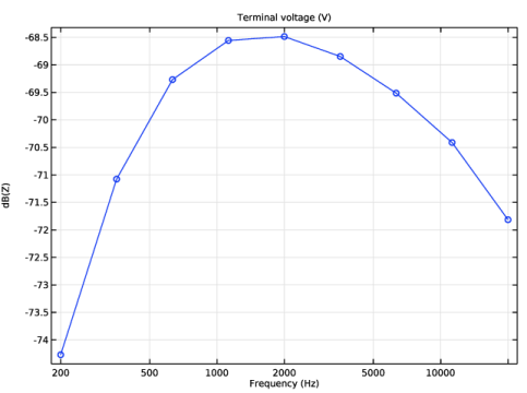
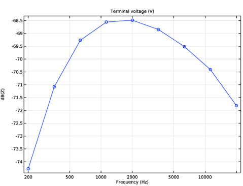
Figure 5 shows the frequency response of the MEMS microphone from 200 Hz to 20 kHz. At the lower frequencies there is roll-off due to the coupling to the electrical circuit (modifying the resistance the electrical circuit changes this behavior). At the high frequencies the response drops off. Because of the small length scale of the model, the mechanical resonances are located at higher frequencies and thus the spectrum is more or less flat in the audio range.
.
Figure 5: Frequency response of the MEMS microphone.
Notes About the COMSOL Implementation
The multiphysics coupling Thermoviscous Acoustics–Structure Boundary does not include the option to set a slip velocity boundary condition in the fluid. Thus, the model uses a manual coupling between the Thermoviscous Acoustics, Frequency Domain and Solid Mechanics physics interfaces. In the Slip Wall node, the Mechanical condition is set to Moving Wall and the velocity input is chosen to be Velocity (solid/lemm1). In the Solid Mechanics interface, a Boundary Load is added on the diaphragm, where the Force per unit area is set to Acoustic slip wall traction per unit area (ta/slw2) picked up from the Slip Wall boundary in the Thermoviscous Acoustics, Frequency Domain interface.
The size of the model makes it advantageous to use an iterative solver, the suggested iterative solver does not include the variables related to the moving mesh. Therefore, a fourth direct preconditioner is added that contains the variables related to the moving mesh.
Reference
1. P. Loeppert and S. Lee, “Sisonic–the first commercialized MEMS microphone,” Solid-state sensors, actuators and microsystems workshop, Hilton Head Island, South Carolina, pp. 27–30, 2006.
Application Library path: Acoustics_Module/Electroacoustic_Transducers/mems_microphone_slip_wall
Modeling Instructions
From the File menu, choose New.
New
In the New window, click  Model Wizard.
Model Wizard
1
In the Model Wizard window, click  3D.
2
In the Select Physics tree, select Acoustics > Thermoviscous Acoustics > Thermoviscous Acoustics, Frequency Domain (ta).
3
Click Add.
4
In the Select Physics tree, select Acoustics > Elastic Waves > Solid Mechanics (Elastic Waves) (solid).
5
Click Add.
6
In the Select Physics tree, select AC/DC > Electric Fields and Currents > Electrostatics (es).
7
Click Add.
8
In the Select Physics tree, select AC/DC > Electrical Circuit (cir).
9
Click Add.
10
In the Select Physics tree, select Mathematics > Deformed Mesh > Moving Mesh > Free Deformation.
11
Click Add.
12
In the Select Physics tree, select Mathematics > Deformed Mesh > Moving Mesh.
13
Click  Study.
14
In the Select Study tree, select Preset Studies for Some Physics Interfaces > Stationary.
15
Global Definitions
Parameters 1
1
In the Model Builder window, under Global Definitions click Parameters 1.
2
In the Settings window for Parameters, locate the Parameters section.
3
Click  Load from File.
4
Geometry 1
1
In the Model Builder window, expand the Component 1 (comp1) > Geometry 1 node, then click Geometry 1.
2
In the Settings window for Geometry, locate the Units section.
3
From the Length unit list, choose µm.
Cylinder 1 (cyl1)
1
In the Geometry toolbar, click  Cylinder.
2
In the Settings window for Cylinder, locate the Size and Shape section.
3
In the Radius text field, type dia_r*1.
4
In the Height text field, type 200[µm].
5
Locate the Position section. In the z text field, type -100[µm].
Diaphragm
1
Right-click Cylinder 1 (cyl1) and choose Duplicate.
2
In the Settings window for Cylinder, locate the Size and Shape section.
3
In the Height text field, type dia_t.
4
Locate the Position section. In the z text field, type 0.
5
In the Label text field, type Diaphragm.
Backplate
1
Right-click Diaphragm and choose Duplicate.
2
In the Settings window for Cylinder, type Backplate in the Label text field.
3
Locate the Size and Shape section. In the Height text field, type back_t.
4
Locate the Position section. In the z text field, type gap+dia_t.
Initial hole
1
Right-click Backplate and choose Duplicate.
2
In the Settings window for Cylinder, locate the Size and Shape section.
3
In the Radius text field, type hole_r.
4
In the Label text field, type Initial hole.
Cylinder 1 (cyl1)
1
In the Model Builder window, click Cylinder 1 (cyl1).
2
In the Settings window for Cylinder, click to expand the Layers section.
3
4
Select the Layers on bottom checkbox.
5
Clear the Layers on side checkbox.
Create an array of holes in a hexagonal lattice structure.
Array 1 (arr1)
1
In the Geometry toolbar, click  Transforms and choose Array.
2
Click the  Wireframe Rendering button in the Graphics toolbar.
3
4
In the Settings window for Array, locate the Size section.
5
From the Array type list, choose Linear.
6
In the Size text field, type 2.
7
Locate the Displacement section. In the x text field, type hole_dist.
Array 2 (arr2)
1
In the Geometry toolbar, click  Transforms and choose Array.
2
Select the objects arr1(1) and arr1(2) only.
3
In the Settings window for Array, locate the Size section.
4
From the Array type list, choose Linear.
5
In the Size text field, type 2.
6
Locate the Displacement section. In the x text field, type hole_dist/2.
7
In the y text field, type sin(pi/3)*hole_dist.
Array 3 (arr3)
1
In the Geometry toolbar, click  Transforms and choose Array.
2
Select the objects arr2(1,1), arr2(1,2), arr2(2,1), and arr2(2,2) only.
3
In the Settings window for Array, locate the Size section.
4
In the x size text field, type 8.
5
In the y size text field, type 8.
6
Locate the Displacement section. In the x text field, type 2*hole_dist.
7
In the y text field, type 2*sin(pi/3)*hole_dist.
8
Locate the Selections of Resulting Entities section. Find the Cumulative selection subsection. Click New.
9
In the New Cumulative Selection dialog, type Holes in the Name text field.
10
Cylinder Selection 1 (cylsel1)
1
In the Geometry toolbar, click  Selections and choose Cylinder Selection.
2
In the Settings window for Cylinder Selection, locate the Geometric Entity Level section.
3
From the Level list, choose Object.
4
Locate the Input Entities section. From the Entities list, choose From selections.
5
6
In the Add dialog, select Holes in the Selections list.
7
8
In the Settings window for Cylinder Selection, locate the Size and Shape section.
9
In the Outer radius text field, type 4*dia_r.
10
In the Inner radius text field, type 0.75*dia_r.
11
Locate the Output Entities section. From the Include entity if list, choose Some vertex inside cylinder.
12
Locate the Resulting Selection section. Clear the Keep selection checkbox.
13
Find the Cumulative selection subsection. Click New.
14
In the New Cumulative Selection dialog, type Holes tmp in the Name text field.
15
Delete Entities 1 (del1)
1
In the Model Builder window, right-click Geometry 1 and choose Delete Entities.
2
In the Settings window for Delete Entities, locate the Entities or Objects to Delete section.
3
From the Selection list, choose Holes tmp.
Array 1 (arr1), Array 2 (arr2), Array 3 (arr3), Cylinder Selection 1 (cylsel1), Delete Entities 1 (del1), Initial hole (cyl4)
1
In the Model Builder window, under Component 1 (comp1) > Geometry 1, Ctrl-click to select Initial hole (cyl4), Array 1 (arr1), Array 2 (arr2), Array 3 (arr3), Cylinder Selection 1 (cylsel1), and Delete Entities 1 (del1).
2
Holes
In the Settings window for Group, type Holes in the Label text field.
Vent 1
1
In the Geometry toolbar, click  Cylinder.
2
In the Settings window for Cylinder, type Vent 1 in the Label text field.
3
Locate the Size and Shape section. In the Radius text field, type vent_r.
4
In the Height text field, type back_t.
5
Locate the Position section. In the x text field, type cos(5*pi/180)*vent_d.
6
In the y text field, type sin(5*pi/180)*vent_d.
7
In the z text field, type gap+dia_t.
8
Locate the Selections of Resulting Entities section. Find the Cumulative selection subsection. Click New.
9
In the New Cumulative Selection dialog, type Vents in the Name text field.
10
Vent 2
1
Right-click Vent 1 and choose Duplicate.
2
In the Settings window for Cylinder, type Vent 2 in the Label text field.
3
Locate the Position section. In the x text field, type cos(15*pi/180)*vent_d.
4
In the y text field, type sin(15*pi/180)*vent_d.
Vent 3
1
Right-click Vent 2 and choose Duplicate.
2
In the Settings window for Cylinder, type Vent 3 in the Label text field.
3
Locate the Position section. In the x text field, type cos(25*pi/180)*vent_d.
4
In the y text field, type sin(25*pi/180)*vent_d.
Vent 1 (cyl5), Vent 2 (cyl6), Vent 3 (cyl7)
1
In the Model Builder window, under Component 1 (comp1) > Geometry 1, Ctrl-click to select Vent 1 (cyl5), Vent 2 (cyl6), and Vent 3 (cyl7).
2
Vents
In the Settings window for Group, type Vents in the Label text field.
Cylinder Selection 2 (cylsel2)
1
In the Geometry toolbar, click  Selections and choose Cylinder Selection.
2
In the Settings window for Cylinder Selection, locate the Size and Shape section.
3
In the Outer radius text field, type 1[mm].
4
Locate the Geometric Entity Level section. From the Level list, choose Object.
5
Locate the Resulting Selection section. Find the Cumulative selection subsection. Click New.
6
In the New Cumulative Selection dialog, type AllCyl in the Name text field.
7
8
In the Settings window for Cylinder Selection, click  Build Selected.
Union 1 (uni1)
1
In the Geometry toolbar, click  Booleans and Partitions and choose Union.
2
In the Settings window for Union, locate the Union section.
3
From the Input objects list, choose AllCyl.
Use a Work Plane and Intersection node to create a 30 degree section of the geometry.
Work Plane 1 (wp1)
1
In the Geometry toolbar, click  Work Plane.
2
In the Settings window for Work Plane, locate the Plane Definition section.
3
In the z-coordinate text field, type -100[µm].
Work Plane 1 (wp1) > Plane Geometry
In the Model Builder window, expand the Component 1 (comp1) > Geometry 1 > Work Plane 1 (wp1) > View 2 node, then click Component 1 (comp1) > Geometry 1 > Work Plane 1 (wp1) > Plane Geometry.
Work Plane 1 (wp1) > Circle 1 (c1)
1
In the Work Plane toolbar, click  Circle.
2
In the Settings window for Circle, locate the Size and Shape section.
3
In the Radius text field, type dia_r.
4
In the Sector angle text field, type 30.
5
In the Work Plane toolbar, click  Build All.
Extrude 1 (ext1)
1
In the Model Builder window, right-click Geometry 1 and choose Extrude.
2
In the Settings window for Extrude, locate the Distances section.
3
Intersection 1 (int1)
1
In the Geometry toolbar, click  Booleans and Partitions and choose Intersection.
2
Select the objects ext1 and uni1 only.
3
In the Settings window for Intersection, click  Build All Objects.
Definitions
Create selections to make it easier to select domains and surfaces.
Diaphragm
1
In the Definitions toolbar, click  Explicit.
2
In the Settings window for Explicit, type Diaphragm in the Label text field.
3
Diaphragm boundaries
1
In the Definitions toolbar, click  Adjacent.
2
In the Settings window for Adjacent, type Diaphragm boundaries in the Label text field.
3
Locate the Input Entities section. Under Input selections, click  Add.
4
In the Add dialog, select Diaphragm in the Input selections list.
5
Slip wall boundaries
1
In the Definitions toolbar, click  Explicit.
2
In the Settings window for Explicit, type Slip wall boundaries in the Label text field.
3
4
Locate the Output Entities section. From the Output entities list, choose Adjacent boundaries.
5
Select the Interior boundaries checkbox.
Large air domain
1
In the Definitions toolbar, click  Explicit.
2
In the Settings window for Explicit, type Large air domain in the Label text field.
3
Air - TA
1
In the Definitions toolbar, click  Union.
2
In the Settings window for Union, type Air - TA in the Label text field.
3
Locate the Input Entities section. Under Selections to add, click  Add.
4
In the Add dialog, in the Selections to add list, choose Large air domain, Holes, and Vents.
5
Symmetry
1
In the Definitions toolbar, click  Explicit.
2
In the Settings window for Explicit, locate the Input Entities section.
3
From the Geometric entity level list, choose Boundary.
4
5
Select the Group by continuous tangent checkbox.
6
In the Label text field, type Symmetry.
All domains - Exterior boundaries
1
In the Definitions toolbar, click  Explicit.
2
In the Settings window for Explicit, locate the Output Entities section.
3
From the Output entities list, choose Adjacent boundaries.
4
Locate the Input Entities section. Select the All domains checkbox.
5
In the Label text field, type All domains - Exterior boundaries.
Top of MPP
1
In the Definitions toolbar, click  Explicit.
2
In the Settings window for Explicit, type Top of MPP in the Label text field.
3
Locate the Input Entities section. From the Geometric entity level list, choose Boundary.
4
5
Select the Group by continuous tangent checkbox.
Air - ACPR
1
In the Definitions toolbar, click  Explicit.
2
In the Settings window for Explicit, type Air - ACPR in the Label text field.
3
Backplate boundaries
1
In the Definitions toolbar, click  Explicit.
2
In the Settings window for Explicit, type Backplate boundaries in the Label text field.
3
4
Locate the Output Entities section. From the Output entities list, choose Adjacent boundaries.
Electrostatics domains
1
In the Definitions toolbar, click  Union.
2
In the Settings window for Union, type Electrostatics domains in the Label text field.
3
Locate the Input Entities section. Under Selections to add, click  Add.
4
In the Add dialog, in the Selections to add list, choose Diaphragm and Air - TA.
5
Add Material
1
In the Materials toolbar, click  Add Material to open the Add Material window.
2
Go to the Add Material window.
3
In the tree, select Built-in > Air and Built-in > Silicon.
4
Click the Add to Component button in the window toolbar.
5
In the Materials toolbar, click  Add Material to close the Add Material window.
Materials
Silicon (mat2)
1
In the Settings window for Material, locate the Geometric Entity Selection section.
2
From the Selection list, choose Diaphragm.
Air (mat1)
1
In the Model Builder window, click Air (mat1).
2
In the Settings window for Material, locate the Geometric Entity Selection section.
3
From the Selection list, choose All domains.
Moving Mesh
Deforming Domain 1
1
In the Model Builder window, expand the Component 1 (comp1) > Moving Mesh node, then click Deforming Domain 1.
2
In the Settings window for Deforming Domain, locate the Domain Selection section.
3
Click  Clear Selection.
4
Set Mesh smoothing type to Laplace which is more efficient for small perturbations to the mesh.
5
Locate the Smoothing section. From the Mesh smoothing type list, choose Laplace.
Component 1 (comp1)
Symmetry/Roller 1
1
In the Moving Mesh toolbar, click  Symmetry/Roller.
2
In the Settings window for Symmetry/Roller, locate the Boundary Selection section.
3
From the Selection list, choose Symmetry.
Thermoviscous Acoustics, Frequency Domain (ta)
1
In the Model Builder window, under Component 1 (comp1) click Thermoviscous Acoustics, Frequency Domain (ta).
2
In the Settings window for Thermoviscous Acoustics, Frequency Domain, locate the Domain Selection section.
3
From the Selection list, choose Air - TA.
Slip Wall 1
In the Physics toolbar, click  Boundaries and choose Slip Wall.
Wall 1
1
In the Model Builder window, click Wall 1.
2
In the Settings window for Wall, locate the Mechanical section.
3
From the Mechanical condition list, choose Slip (perfect).
4
Locate the Thermal section. From the Thermal condition list, choose Adiabatic.
Slip Wall - MPP
1
In the Model Builder window, under Component 1 (comp1) > Thermoviscous Acoustics, Frequency Domain (ta) click Slip Wall 1.
2
In the Settings window for Slip Wall, type Slip Wall - MPP in the Label text field.
3
Locate the Boundary Selection section. From the Selection list, choose Slip wall boundaries.
Slip Wall - Diaphragm
1
In the Physics toolbar, click  Boundaries and choose Slip Wall.
2
In the Settings window for Slip Wall, type Slip Wall - Diaphragm in the Label text field.
3
Locate the Boundary Selection section. From the Selection list, choose Diaphragm boundaries.
4
Locate the Mechanical section. From the Mechanical condition list, choose Moving wall.
5
From the uw list, choose Velocity (solid/lemm1).
Manually couple to the velocity of the diaphragm.
Symmetry 1
1
In the Physics toolbar, click  Boundaries and choose Symmetry.
2
In the Settings window for Symmetry, locate the Boundary Selection section.
3
From the Selection list, choose Symmetry.
Pressure (Adiabatic) 1
1
In the Physics toolbar, click  Boundaries and choose Pressure (Adiabatic).
2
3
In the Settings window for Pressure (Adiabatic), locate the Pressure section.
4
In the pbnd text field, type linper(1[Pa]).
Wall 2
1
In the Physics toolbar, click  Boundaries and choose Wall.
2
Solid Mechanics (solid)
1
In the Model Builder window, under Component 1 (comp1) click Solid Mechanics (solid).
2
In the Settings window for Solid Mechanics, locate the Domain Selection section.
3
From the Selection list, choose Diaphragm.
Fixed Constraint 1
1
In the Physics toolbar, click  Boundaries and choose Fixed Constraint.
2
In the Settings window for Fixed Constraint, locate the Boundary Selection section.
3
From the Selection list, choose All domains - Exterior boundaries.
Symmetry 1
1
In the Physics toolbar, click  Boundaries and choose Symmetry.
2
In the Settings window for Symmetry, locate the Boundary Selection section.
3
From the Selection list, choose Symmetry.
Add a Boundary Load to make the manual coupling to the Thermoviscous Acoustics.
Boundary Load 1
1
In the Physics toolbar, click  Boundaries and choose Boundary Load.
2
3
In the Settings window for Boundary Load, locate the Force section.
4
From the Load type list, choose Force per deformed area.
5
From the fa list, choose Acoustic slip wall traction per unit area (ta/slw2).
Electrostatics (es)
1
In the Model Builder window, under Component 1 (comp1) click Electrostatics (es).
2
In the Settings window for Electrostatics, locate the Domain Selection section.
3
From the Selection list, choose Electrostatics domains.
Charge Conservation in Solids 1
1
In the Physics toolbar, click  Domains and choose Charge Conservation in Solids.
2
In the Settings window for Charge Conservation in Solids, locate the Domain Selection section.
3
From the Selection list, choose Diaphragm.
Ground 1
1
In the Physics toolbar, click  Boundaries and choose Ground.
2
Boundary Terminal 1
1
In the Physics toolbar, click  Boundaries and choose Boundary Terminal.
2
In the Settings window for Boundary Terminal, locate the Boundary Selection section.
3
From the Selection list, choose Backplate boundaries.
4
Locate the Terminal section. From the Terminal type list, choose Circuit.
Symmetry Plane 1
1
In the Physics toolbar, click  Boundaries and choose Symmetry Plane.
2
In the Settings window for Symmetry Plane, locate the Boundary Selection section.
3
From the Selection list, choose Symmetry.
Electrical Circuit (cir)
In the Model Builder window, under Component 1 (comp1) click Electrical Circuit (cir).
External I vs. U 1 (IvsU1)
1
In the Electrical Circuit toolbar, click  External I vs. U.
2
In the Settings window for External I vs. U, locate the External Device section.
3
From the V list, choose Terminal voltage (es/term1).
4
Locate the Node Connections section. In the table, enter the following settings:
Resistor 1 (R1)
1
In the Electrical Circuit toolbar, click  Resistor.
2
In the Settings window for Resistor, locate the Node Connections section.
3
4
Locate the Device Parameters section. In the R text field, type 10[Gohm].
Voltage Source 1 (V1)
1
In the Electrical Circuit toolbar, click  Voltage Source.
2
In the Settings window for Voltage Source, locate the Device Parameters section.
3
In the vsrc text field, type 1[V].
4
Locate the Node Connections section. In the table, enter the following settings:
Multiphysics
Electromechanics, Solid 1 (eme1)
In the Model Builder window, under Component 1 (comp1) right-click Multiphysics and choose Electromechanics, Solid.
Thermoviscous Acoustic–Structure Boundary 1 (tsb1)
1
In the Model Builder window, right-click Multiphysics and choose Thermoviscous Acoustic–Structure Boundary.
2
Mesh 1
Size 1
In the Model Builder window, under Component 1 (comp1) right-click Mesh 1 and choose Size.
Size
1
In the Settings window for Size, locate the Element Size section.
2
From the Predefined list, choose Finer.
Size - Holes
1
In the Model Builder window, click Size 1.
2
In the Settings window for Size, locate the Geometric Entity Selection section.
3
From the Geometric entity level list, choose Domain.
4
From the Selection list, choose Holes.
5
Locate the Element Size section. Click the Custom button.
6
Locate the Element Size Parameters section.
7
Select the Maximum element size checkbox. In the associated text field, type hole_r/1.5.
8
In the Label text field, type Size - Holes.
Size - Vents
1
Right-click Size - Holes and choose Duplicate.
2
In the Settings window for Size, type Size - Vents in the Label text field.
3
Locate the Geometric Entity Selection section. From the Selection list, choose Vents.
4
Locate the Element Size Parameters section. In the Maximum element size text field, type vent_r/1.5.
Free Triangular 1
1
In the Mesh toolbar, click  More Generators and choose Free Triangular.
2
In the Settings window for Free Triangular, locate the Boundary Selection section.
3
From the Selection list, choose Top of MPP.
4
Click  Build Selected.
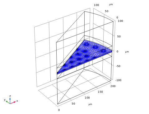
The triangular mesh should be as the following figure.
Swept - Gap and diaphragm
1
In the Mesh toolbar, click  Swept.
2
In the Settings window for Swept, type Swept - Gap and diaphragm in the Label text field.
3
Locate the Domain Selection section. From the Geometric entity level list, choose Domain.
4
Distribution 1
1
Right-click Swept - Gap and diaphragm and choose Distribution.
2
3
In the Settings window for Distribution, locate the Distribution section.
4
From the Distribution type list, choose Predefined.
5
In the Element ratio text field, type 5.
6
Select the Symmetric distribution checkbox.
Distribution 2
1
Right-click Distribution 1 and choose Duplicate.
2
In the Settings window for Distribution, locate the Distribution section.
3
From the Distribution type list, choose Fixed number of elements.
4
5
In the Number of elements text field, type 2.
Swept - Holes
1
In the Mesh toolbar, click  Swept.
2
In the Settings window for Swept, type Swept - Holes in the Label text field.
3
Locate the Domain Selection section. From the Geometric entity level list, choose Domain.
4
From the Selection list, choose Holes.
Distribution 1
1
Right-click Swept - Holes and choose Distribution.
2
In the Settings window for Distribution, locate the Distribution section.
3
From the Distribution type list, choose Predefined.
4
Select the Symmetric distribution checkbox.
5
In the Element ratio text field, type 5.
Swept - Vents
1
In the Model Builder window, right-click Swept - Holes and choose Duplicate.
2
In the Settings window for Swept, type Swept - Vents in the Label text field.
3
Locate the Domain Selection section. From the Selection list, choose Vents.
4
Click  Build Selected.
Free Tetrahedral 1
1
In the Mesh toolbar, click  Free Tetrahedral.
2
In the Settings window for Free Tetrahedral, locate the Domain Selection section.
3
From the Geometric entity level list, choose Domain.
4
5
Click  Build All.
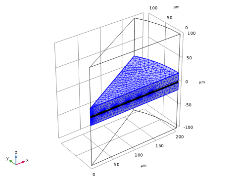
The finalized mesh should be as the following figure.
Swept 4
1
In the Mesh toolbar, click  Swept.
2
In the Settings window for Swept, locate the Domain Selection section.
3
From the Geometric entity level list, choose Domain.
4
5
Click  Build All.
Study 1
Step 2: Frequency-Domain Perturbation
1
In the Model Builder window, expand the Study 1 node.
2
Right-click Study 1 and choose More Study Steps > Frequency Domain > Frequency-Domain Perturbation.
3
In the Settings window for Frequency-Domain Perturbation, locate the Study Settings section.
4
In the Frequencies text field, type 10^{range(log10(200),1/4,log10(20000))}.
5
From the Tolerance list, choose User controlled.
6
In the Relative tolerance text field, type 1e-3.
Solution 1 (sol1)
1
In the Study toolbar, click  Show Default Solver.
2
In the Model Builder window, expand the Solution 1 (sol1) node.
3
In the Model Builder window, expand the Study 1 > Solver Configurations > Solution 1 (sol1) > Stationary Solver 2 node.
4
Right-click Study 1 > Solver Configurations > Solution 1 (sol1) > Stationary Solver 2 > Suggested Iterative Solver (GMRES with Direct Precond.) (tsb1_eme1) and choose Enable.
5
In the Study toolbar, click  Compute.
Results
In the Model Builder window, expand the Results node.
Sector 3D 1
1
In the Model Builder window, expand the Results > Datasets node.
2
Right-click Results > Datasets and choose More 3D Datasets > Sector 3D.
3
In the Settings window for Sector 3D, locate the Symmetry section.
4
In the Number of sectors text field, type 12.
5
From the Sectors to include list, choose Manual.
6
In the Number of sectors to include text field, type 12.
7
From the Transformation list, choose Rotation and reflection.
8
Sector 3D 2
1
Right-click Sector 3D 1 and choose Duplicate.
2
In the Settings window for Sector 3D, locate the Symmetry section.
3
In the Number of sectors text field, type 12.
4
In the Number of sectors to include text field, type 9.
5
In the Start sector text field, type -2.
6
Frequency Response
1
In the Results toolbar, click  1D Plot Group.
2
In the Settings window for 1D Plot Group, type Frequency Response in the Label text field.
Octave Band 1
1
In the Frequency Response toolbar, click  More Plots and choose Octave Band.
2
In the Settings window for Octave Band, locate the Selection section.
3
From the Geometric entity level list, choose Global.
4
Locate the y-Axis Data section. In the Expression text field, type es.V0_1.
5
Click  Replace Expression.
6
In the Amplitude reference text field, type 1/sqrt(2).
7
Locate the Plot section. From the Quantity list, choose Continuous power spectral density.
8
Click to expand the Coloring and Style section. Find the Line markers subsection. From the Marker list, choose Circle.
9
In the Frequency Response toolbar, click  Plot.
Acoustic Pressure
1
In the Results toolbar, click  3D Plot Group.
2
In the Settings window for 3D Plot Group, type Acoustic Pressure in the Label text field.
3
Locate the Color Legend section. Select the Show units checkbox.
TA
1
Right-click Acoustic Pressure and choose Surface.
2
In the Settings window for Surface, type TA in the Label text field.
3
Locate the Coloring and Style section. From the Color table list, choose Wave.
4
From the Scale list, choose Linear symmetric.
5
In the Acoustic Pressure toolbar, click  Plot.
Acoustic Velocity
1
In the Results toolbar, click  3D Plot Group.
2
In the Settings window for 3D Plot Group, type Acoustic Velocity in the Label text field.
3
Locate the Color Legend section. Select the Show units checkbox.
Surface 1
1
Right-click Acoustic Velocity and choose Surface.
2
In the Settings window for Surface, locate the Expression section.
3
In the Expression text field, type ta.v_rms.
4
From the Unit list, choose mm/s.
5
In the Acoustic Velocity toolbar, click  Plot.