
|
|
|
|
-
|
|
1
|
|
2
|
|
3
|
Click Add.
|
|
4
|
Click
|
|
5
|
|
6
|
Click
|
|
1
|
|
2
|
|
3
|
|
4
|
|
5
|
Browse to the model’s Application Libraries folder and double-click the file magnetic_circuit_topology_optimization_geom_sequence.mph.
|
|
6
|
|
1
|
|
2
|
|
1
|
|
2
|
|
3
|
|
4
|
Browse to the model’s Application Libraries folder and double-click the file magnetic_circuit_topology_optimization_model_parameters.txt.
|
|
1
|
|
2
|
Go to the Add Material window.
|
|
3
|
|
4
|
Click the Add to Global Materials button in the window toolbar.
|
|
5
|
|
1
|
In the Model Builder window, under Global Definitions right-click Materials and choose Blank Material.
|
|
2
|
|
3
|
Click to expand the Material Properties section. In the Material properties tree, select Basic Properties > Electric Conductivity.
|
|
4
|
Click
|
|
5
|
|
6
|
Click
|
|
7
|
In the Material properties tree, select Electromagnetic Models > Remanent Flux Density > Recoil permeability (murec).
|
|
8
|
Click
|
|
9
|
Locate the Material Contents section. In the table, enter the following settings:
|
|
1
|
|
2
|
In the Settings window for Analytic, type Equivalent mur of mat1, Soft Iron (With Losses) in the Label text field.
|
|
3
|
|
4
|
Locate the Definition section. In the Expression text field, type sqrt(Bx^2+By^2+eps[T^2])/mat1.BHCurve.BH_inv(sqrt(Bx^2+By^2+eps[T^2]))/mu0_const.
|
|
5
|
|
6
|
|
8
|
Locate the Plot Parameters section. In the table, enter the following settings:
|
|
9
|
Click
|
|
1
|
|
2
|
|
3
|
|
4
|
|
5
|
|
6
|
|
7
|
In the Show More Options dialog, in the tree, select the checkbox for the node General > Variable Utilities, so that the Expression Operator becomes accessible.
|
|
8
|
Click OK.
|
|
1
|
|
2
|
|
3
|
|
4
|
|
5
|
Locate the Definition section. In the Expression text field, type int_BL(if((z>(z0-h_coil/2))*(z<(z0+h_coil/2)),-mf.Br*N0/(w_coil*h_coil),0)).
|
|
1
|
|
2
|
|
3
|
|
4
|
Locate the Source Selection section. From the Selection list, choose Voice Coil Center at Resting Position.
|
|
5
|
|
1
|
|
2
|
|
3
|
|
4
|
Locate the Source Selection section. From the Selection list, choose Voice Coil Center Measuring Points.
|
|
1
|
|
2
|
|
3
|
|
4
|
|
5
|
|
1
|
|
2
|
|
3
|
|
4
|
|
5
|
In the text field, type SIMPp.
|
|
6
|
|
7
|
|
8
|
|
10
|
|
11
|
|
1
|
In the Model Builder window, under Component 1 (comp1) right-click Materials and choose More Materials > Material Link.
|
|
2
|
|
3
|
|
1
|
|
2
|
|
3
|
|
4
|
|
1
|
|
2
|
|
3
|
|
1
|
|
2
|
In the Settings window for Ampère’s Law in Solids, type Topology Optimization in the Label text field.
|
|
3
|
|
4
|
Locate the Constitutive Relation B-H section. From the μr list, choose User defined. In the associated text field, type 1+dtopo1.theta_p*(mur1(mf.Br,mf.Bz)-1).
|
|
1
|
|
2
|
|
3
|
|
4
|
Locate the Constitutive Relation B-H section. From the Magnetization model list, choose Remanent flux density.
|
|
5
|
Specify the e vector as
|
|
1
|
|
2
|
|
3
|
|
4
|
|
1
|
|
2
|
|
3
|
Click the Custom button.
|
|
4
|
Locate the Element Size Parameters section.
|
|
5
|
|
1
|
|
2
|
|
3
|
|
4
|
|
5
|
|
6
|
Locate the Element Size Parameters section.
|
|
7
|
|
1
|
|
2
|
|
3
|
|
4
|
Click
|
|
1
|
|
2
|
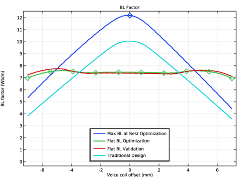
In the Settings window for Study, type Study 1 - Max BL at Rest Optimization in the Label text field.
|
|
1
|
|
2
|
|
3
|
|
4
|
Click Add Expression in the upper-right corner of the Objective Function section. From the menu, choose Component 1 (comp1) > Definitions > comp1.obj_1 - Point Probe - Objective 1 - Wb/m.
|
|
5
|
|
6
|
Find the Objective settings subsection. From the Objective scaling list, choose Initial solution based.
|
|
7
|
Click Add Expression in the upper-right corner of the Constraints section. From the menu, choose Component 1 (comp1) > Definitions > Density Model 1 > Global > comp1.dtopo1.theta_avg - Average material volume factor - 1.
|
|
8
|
Locate the Constraints section. In the table, enter the following settings:
|
|
9
|
|
10
|
|
11
|
|
12
|
|
13
|
Select the Plot checkbox.
|
|
15
|
|
1
|
|
2
|
|
1
|
In the Settings window for Filter, type Filter - Max BL at Rest Optimization in the Label text field.
|
|
2
|
Locate the Expression section. In the Expression text field, type if(isnan(dtopo1.theta_c),NaN,dtopo1.theta).
|
|
1
|
|
2
|
|
1
|
|
2
|
|
3
|
|
1
|
|
2
|
|
3
|
Select the Manual color range checkbox.
|
|
4
|
|
5
|
|
1
|
|
2
|
Drag and drop on Topology Optimization.
|
|
1
|
|
2
|
|
1
|
|
2
|
|
3
|
|
1
|
|
2
|
|
3
|
|
4
|
|
5
|
|
1
|
|
2
|
Go to the Add Study window.
|
|
3
|
|
4
|
Click the Add Study button in the window toolbar.
|
|
5
|
|
1
|
|
2
|
|
3
|
|
4
|
Click Add Expression in the upper-right corner of the Objective Function section. From the menu, choose Component 1 (comp1) > Definitions > comp1.obj_2 - Point Probe - Objective 2 - Wb/m.
|
|
5
|
|
6
|
Find the Objective settings subsection. From the Objective scaling list, choose Initial solution based.
|
|
7
|
Click Add Expression in the upper-right corner of the Constraints section. From the menu, choose Component 1 (comp1) > Definitions > Density Model 1 > Global > comp1.dtopo1.theta_avg - Average material volume factor - 1.
|
|
8
|
Click Add Expression in the upper-right corner of the Constraints section. From the menu, choose Component 1 (comp1) > Definitions > comp1.std1 - Standard deviation - Wb/m.
|
|
9
|
Locate the Constraints section. In the table, enter the following settings:
|
|
10
|
|
11
|
|
12
|
|
13
|
|
14
|
Select the Plot checkbox.
|
|
16
|
|
1
|
|
2
|
Locate the Expression section. In the Expression text field, type if(isnan(dtopo1.theta_c),NaN,dtopo1.theta).
|
|
1
|
|
2
|
|
3
|
|
1
|
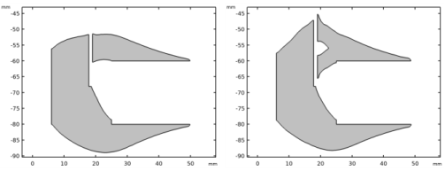
In the Model Builder window, expand the Results > Topology Optimization node, then click Threshold 1.
|
|
2
|
|
3
|
|
4
|
|
1
|
|
2
|
|
3
|
|
1
|
|
2
|
|
3
|
Select the Manual color range checkbox.
|
|
4
|
|
5
|
|
1
|
|
2
|
Drag and drop on Topology Optimization.
|
|
1
|
|
2
|
|
1
|
|
2
|
|
3
|
|
1
|
|
2
|
|
3
|
|
4
|
|
5
|
|
1
|
|
2
|
|
1
|
|
2
|
|
3
|
|
1
|
|
2
|
|
3
|
|
4
|
|
5
|
Click
|
|
1
|
|
2
|
|
3
|
|
4
|
|
5
|
Click
|
|
1
|
|
2
|
In the Settings window for Integration, type Area to Obtain the BL Factor 2 in the Label text field.
|
|
3
|
|
4
|
Locate the Source Selection section. From the Selection list, choose Voice Coil Possible Locations (Import 2).
|
|
5
|
|
1
|
|
2
|
|
3
|
|
4
|
|
5
|
Locate the Definition section. In the Expression text field, type int_BL2(if((z>(z0-h_coil/2))*(z<(z0+h_coil/2)),-mf2.Br*N0/(w_coil*h_coil),0)).
|
|
1
|
In the Model Builder window, under Component 2: Verification (comp2) right-click Materials and choose More Materials > Material Link.
|
|
2
|
|
3
|
Locate the Geometric Entity Selection section. From the Selection list, choose Design Space (Import 1).
|
|
1
|
|
2
|
|
3
|
|
4
|
|
1
|
|
2
|
Go to the Add Physics window.
|
|
3
|
|
4
|
Find the Physics interfaces in study subsection. In the table, clear the Solve checkboxes for Study 1 - Max BL at Rest Optimization and Study 2 - Flat BL Optimization.
|
|
5
|
Click the Add to Component 2: Verification button in the window toolbar.
|
|
6
|
|
1
|
|
2
|
|
3
|
|
4
|
|
1
|
|
2
|
|
3
|
|
4
|
Locate the Constitutive Relation B-H section. From the Magnetization model list, choose Remanent flux density.
|
|
5
|
Specify the e vector as
|
|
1
|
|
2
|
|
3
|
|
4
|
|
1
|
|
2
|
|
3
|
Click the Custom button.
|
|
4
|
Locate the Element Size Parameters section.
|
|
5
|
|
1
|
|
2
|
|
3
|
|
4
|
|
5
|
|
6
|
Locate the Element Size Parameters section.
|
|
7
|
|
1
|
|
2
|
Go to the Add Study window.
|
|
3
|
|
4
|
Find the Physics interfaces in study subsection. In the table, clear the Solve checkbox for Magnetic Fields (mf).
|
|
5
|
Click the Add Study button in the window toolbar.
|
|
6
|
|
1
|
|
2
|
|
3
|
|
4
|
|
5
|
|
1
|
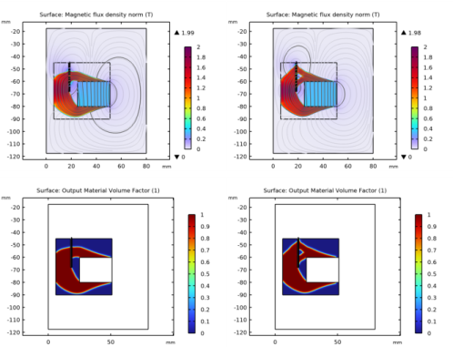
In the Model Builder window, expand the Results > Topology Optimization node, then click Results > Magnetic Flux Density (mf2).
|
|
2
|
|
3
|
|
1
|
|
2
|
|
3
|
Select the Manual color range checkbox.
|
|
4
|
|
5
|
|
6
|
|
1
|
|
2
|
Drag and drop on Topology Optimization.
|
|
1
|
In the Model Builder window, under Results > Topology Optimization, Ctrl-click to select Output material volume factor 2 and Threshold 2.
|
|
2
|
Right-click and choose Delete.
|
|
1
|
|
2
|
|
1
|
In the Model Builder window, under Results > Datasets, Ctrl-click to select Study 3 - Flat BL Validation/Solution 3 (4) (sol3), Revolution 2D 1, and Filter.
|
|
2
|
Right-click and choose Delete.
|
|
1
|
|
2
|
|
3
|
|
4
|
Browse to the model’s Application Libraries folder and double-click the file magnetic_circuit_topology_optimization_traditional_bl.txt.
|
|
1
|
|
2
|
|
3
|
Locate the Plot Settings section.
|
|
4
|
|
5
|
|
6
|
|
7
|
|
8
|
|
1
|
|
2
|
|
3
|
|
4
|
|
5
|
|
6
|
|
7
|
|
8
|
|
9
|
|
10
|
|
11
|
|
12
|
|
1
|
|
2
|
|
3
|
|
4
|
Locate the Legends section. Find the Prefix and suffix subsection. In the Prefix text field, type Flat BL Optimization.
|
|
5
|
|
1
|
|
2
|
|
3
|
|
4
|
Locate the Selection section. From the Selection list, choose Voice Coil Center Possible Locations (Import 2).
|
|
5
|
|
6
|
Locate the Legends section. Find the Prefix and suffix subsection. In the Prefix text field, type Flat BL Validation.
|
|
7
|
|
1
|
|
2
|
|
3
|
Clear the Show point checkbox.
|
|
4
|
|
1
|
|
2
|
|
3
|
|
4
|
|
5
|
|
6
|
|
8
|
|
9
|
|
1
|
|
2
|
|
3
|
|
4
|
|
5
|
|
6
|
|
7
|
Click to expand the Coloring and Style section. Find the Line style subsection. From the Line list, choose None.
|
|
8
|
|
9
|
|
10
|
|
11
|
|
1
|
|
2
|
|
3
|
|
4
|
|
5
|
|
6
|
|
7
|
Click Define custom colors.
|
|
9
|
Click Add to custom colors.
|
|
10
|
|
11
|
|
1
|
|
2
|
|
3
|
|
1
|
|
2
|
|
3
|
|
4
|
|
5
|
|
6
|
|
1
|
|
2
|
|
3
|
|
4
|
|
5
|
|
6
|
|
1
|
|
2
|
|
3
|
|
4
|
|
6
|
|
7
|
|
8
|
|
1
|
|
2
|
Click
|
|
1
|
|
2
|
|
3
|
|
1
|
|
2
|
|
3
|
Click
|
|
4
|
Browse to the model’s Application Libraries folder and double-click the file magnetic_circuit_topology_optimization_geom_parameters.txt.
|
|
1
|
|
2
|
|
3
|
|
4
|
|
5
|
|
6
|
Click
|
|
1
|
|
2
|
In the Settings window for Rectangle, type Design Space with Magnet and Coil Gap in the Label text field.
|
|
3
|
|
4
|
|
5
|
|
6
|
|
7
|
Click
|
|
1
|
|
2
|
|
3
|
|
4
|
|
5
|
|
6
|
|
7
|
Click
|
|
1
|
|
2
|
|
3
|
Select the object r2 only.
|
|
4
|
Locate the Difference section. Click to select the
|
|
5
|
Select the object r3 only.
|
|
6
|
Locate the Selections of Resulting Entities section. Select the Resulting objects selection checkbox.
|
|
7
|
Click
|
|
1
|
|
2
|
|
3
|
|
4
|
|
5
|
|
6
|
|
7
|
Locate the Selections of Resulting Entities section. Select the Resulting objects selection checkbox.
|
|
8
|
Click
|
|
1
|
|
2
|
|
3
|
|
4
|
|
5
|
|
6
|
|
7
|
|
8
|
Click to expand the Layers section. In the table, enter the following settings:
|
|
9
|
Select the Layers on top checkbox.
|
|
10
|
Locate the Selections of Resulting Entities section. Select the Resulting objects selection checkbox.
|
|
11
|
Click
|
|
1
|
|
2
|
In the Settings window for Line Segment, type Voice Coil Center Possible Locations in the Label text field.
|
|
3
|
|
4
|
|
5
|
|
6
|
|
7
|
|
8
|
|
9
|
Locate the Selections of Resulting Entities section. Select the Resulting objects selection checkbox.
|
|
10
|
Click
|
|
1
|
|
2
|
|
3
|
|
4
|
|
5
|
Click
|
|
1
|
|
2
|
|
3
|
Select the object pt1 only.
|
|
4
|
|
5
|
|
6
|
Locate the Selections of Resulting Entities section. Select the Resulting objects selection checkbox.
|
|
7
|
|
8
|
Click
|
|
1
|
|
2
|
In the Settings window for Point, type Voice Coil Center at Resting Position in the Label text field.
|
|
3
|
|
4
|
|
5
|
Locate the Selections of Resulting Entities section. Select the Resulting objects selection checkbox.
|
|
6
|
Click
|
|
1
|
|
2
|
|
1
|
|
2
|
|
3
|
|
4
|
|
5
|
Click OK.
|
|
1
|
|
2
|
|
3
|
|
4
|
|
5
|
Click OK.
|
|
6
|
|
7
|
|
8
|
|
9
|
Click OK.
|