|
|
|
|
•
|
|
•
|
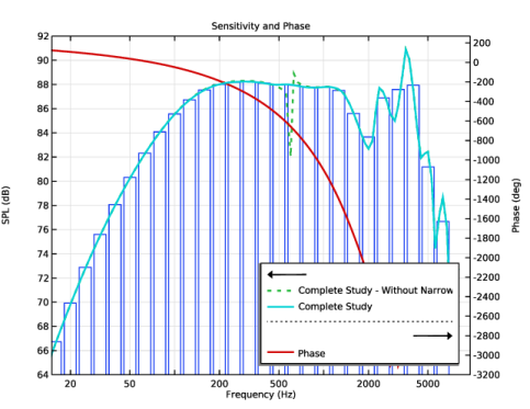
(Optional) Set up a study considering all the physics but disable the Narrow Region Acoustics features.
|
|
1
|
|
2
|
|
3
|
Click Add.
|
|
4
|
In the Select Physics tree, select Acoustics > Acoustic–Structure Interaction > Acoustic–Solid Interaction, Frequency Domain.
|
|
5
|
Click Add.
|
|
6
|
Click
|
|
7
|
|
8
|
Click
|
|
1
|
|
2
|
Browse to the model’s Application Libraries folder and double-click the file loudspeaker_driver_geom_sequence.mph.
|
|
3
|
|
4
|
|
1
|
|
2
|
|
1
|
|
2
|
|
4
|
|
1
|
|
2
|
|
4
|
|
1
|
|
2
|
|
4
|
|
1
|
|
2
|
|
4
|
|
1
|
|
2
|
|
4
|
|
1
|
|
2
|
|
4
|
|
1
|
|
2
|
|
4
|
|
1
|
|
2
|
|
1
|
|
2
|
|
1
|
|
2
|
|
3
|
|
4
|
|
5
|
Click OK.
|
|
6
|
|
7
|
|
8
|
In the Add dialog, in the Selections to subtract list, choose Soft Iron, Composite, Cloth, Foam, Coil, Glass Fiber, and Generic Ferrite.
|
|
9
|
Click OK.
|
|
1
|
|
2
|
|
3
|
|
4
|
In the Add dialog, in the Selections to add list, choose Composite, Cloth, Foam, Coil, and Glass Fiber.
|
|
5
|
Click OK.
|
|
1
|
|
2
|
|
3
|
|
4
|
|
5
|
Click OK.
|
|
1
|
|
2
|
|
3
|
|
4
|
|
5
|
|
6
|
|
1
|
|
2
|
|
3
|
|
4
|
|
5
|
Click OK.
|
|
6
|
|
7
|
|
8
|
|
9
|
Click OK.
|
|
1
|
|
2
|
|
3
|
|
4
|
|
1
|
|
2
|
|
3
|
|
1
|
|
2
|
|
1
|
|
2
|
Go to the Add Material window.
|
|
3
|
|
4
|
Click the Add to Component button in the window toolbar.
|
|
5
|
|
6
|
Click the Add to Component button in the window toolbar.
|
|
1
|
|
2
|
|
3
|
|
4
|
|
1
|
In the Material Browser window, In the ribbon make sure to select the Materials tab and then click the Browse Materials icon.
|
|
2
|
click
|
|
3
|
Browse to the model’s Application Libraries folder and double-click the file loudspeaker_driver_materials.mph.
|
|
4
|
Click
|
|
1
|
Go to the Add Material window.
|
|
2
|
|
3
|
Click the Add to Component button in the window toolbar.
|
|
4
|
|
5
|
Click the Add to Component button in the window toolbar.
|
|
6
|
|
7
|
Click the Add to Component button in the window toolbar.
|
|
8
|
|
9
|
Click the Add to Component button in the window toolbar.
|
|
10
|
|
11
|
Click the Add to Component button in the window toolbar.
|
|
12
|
|
13
|
Click the Add to Component button in the window toolbar.
|
|
14
|
|
1
|
|
2
|
|
1
|
|
2
|
|
3
|
|
1
|
|
2
|
|
3
|
|
1
|
|
2
|
|
3
|
|
1
|
|
2
|
|
3
|
|
1
|
|
2
|
|
3
|
|
1
|
|
2
|
|
3
|
|
1
|
|
2
|
In the Settings window for Ampère’s Law in Solids, type Ampère's Law in Solids - Generic Ferrite in the Label text field.
|
|
3
|
|
4
|
Locate the Constitutive Relation B-H section. From the Magnetization model list, choose Remanent flux density.
|
|
5
|
Specify the e vector as
|
|
1
|
|
2
|
In the Settings window for Ampère’s Law in Solids, type Ampère's Law in Solids - Soft Iron in the Label text field.
|
|
3
|
|
4
|
|
1
|
|
2
|
|
3
|
|
4
|
|
1
|
|
2
|
|
3
|
|
4
|
|
5
|
|
6
|
From the list, choose User defined.
|
|
7
|
|
8
|
|
9
|
|
10
|
|
1
|
In the Model Builder window, under Component 1 (comp1) click Pressure Acoustics, Frequency Domain (acpr).
|
|
2
|
In the Settings window for Pressure Acoustics, Frequency Domain, locate the Domain Selection section.
|
|
3
|
|
1
|
|
3
|
In the Settings window for Exterior Field Calculation, locate the Exterior Field Calculation section.
|
|
4
|
|
1
|
|
3
|
|
4
|
|
5
|
|
1
|
|
2
|
|
3
|
Click
|
|
5
|
|
1
|
|
2
|
|
3
|
|
1
|
|
2
|
|
3
|
Click
|
|
4
|
|
5
|
|
1
|
|
2
|
|
3
|
Click
|
|
4
|
|
5
|
|
1
|
|
2
|
|
3
|
Click
|
|
4
|
|
5
|
|
1
|
|
1
|
|
2
|
|
3
|
Select the Only use Lorentz force checkbox.
|
|
4
|
|
1
|
|
2
|
|
3
|
|
1
|
|
2
|
|
3
|
Click the Custom button.
|
|
4
|
|
5
|
|
6
|
|
1
|
|
3
|
|
4
|
Click the Custom button.
|
|
5
|
Locate the Element Size Parameters section.
|
|
6
|
|
1
|
|
2
|
|
3
|
Click
|
|
5
|
|
6
|
Locate the Element Size Parameters section.
|
|
7
|
|
1
|
|
2
|
|
3
|
Click
|
|
5
|
|
6
|
Locate the Element Size Parameters section.
|
|
7
|
|
1
|
|
3
|
|
4
|
|
1
|
|
3
|
|
4
|
|
5
|
Click
|
|
1
|
|
2
|
|
3
|
|
5
|
|
1
|
|
1
|
|
3
|
|
4
|
|
5
|
Click
|
|
6
|
|
1
|
|
2
|
|
3
|
|
1
|
|
2
|
|
3
|
In the Solve for column of the table, under Component 1 (comp1), clear the checkbox for Solid Mechanics (solid).
|
|
1
|
In the Study toolbar, click
|
|
2
|
|
3
|
|
4
|
Click
|
|
5
|
|
6
|
|
7
|
|
8
|
|
9
|
Click Add.
|
|
10
|
In the Settings window for Frequency-Domain Perturbation, locate the Physics and Variables Selection section.
|
|
11
|
In the Solve for column of the table, under Component 1 (comp1), clear the checkboxes for Pressure Acoustics, Frequency Domain (acpr) and Solid Mechanics (solid).
|
|
12
|
|
1
|
|
2
|
|
3
|
|
4
|
Locate the Data section. From the Dataset list, choose Study 1 - Magnetic Fields/Solution Store 1 (sol2).
|
|
1
|
|
2
|
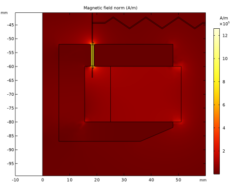
In the Settings window for Surface, click Replace Expression in the upper-right corner of the Expression section. From the menu, choose Component 1 (comp1) > Magnetic Fields > Magnetic > mf.normH - Magnetic field norm - A/m.
|
|
3
|
|
4
|
|
1
|
|
2
|
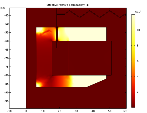
In the Settings window for 2D Plot Group, type Effective Relative Permeability in the Label text field.
|
|
1
|
|
2
|
|
3
|
|
4
|
Select the Description checkbox. In the associated text field, type Effective relative permeability.
|
|
5
|
|
1
|
|
2
|
|
3
|
|
4
|
|
5
|
Locate the Expressions section. In the table, enter the following settings:
|
|
6
|
|
7
|
Click
|
|
1
|
|
2
|
|
3
|
|
1
|
|
2
|
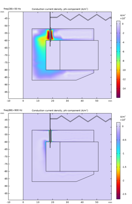
In the Settings window for Surface, click Replace Expression in the upper-right corner of the Expression section. From the menu, choose Component 1 (comp1) > Magnetic Fields > Currents and charge > Conduction current density (spatial frame) - A/m² > mf.Jiphi - Conduction current density, phi-component.
|
|
3
|
|
4
|
|
5
|
|
1
|
|
2
|
|
3
|
|
4
|
|
1
|
|
2
|
|
3
|
|
1
|
|
2
|
|
4
|
|
5
|
|
1
|
|
1
|
|
2
|
Go to the Add Study window.
|
|
3
|
|
4
|
Click the Add Study button in the window toolbar.
|
|
5
|
|
1
|
In the Model Builder window, under Study 1 - Magnetic Fields, Ctrl-click to select Step 1: Stationary and Step 2: Frequency-Domain Perturbation.
|
|
2
|
Right-click and choose Copy.
|
|
1
|
|
2
|
|
3
|
|
1
|
In the Model Builder window, under Study 2 - Complete Model click Step 2: Frequency-Domain Perturbation.
|
|
2
|
In the Settings window for Frequency-Domain Perturbation, locate the Physics and Variables Selection section.
|
|
3
|
In the Solve for column of the table, under Component 1 (comp1), select the checkboxes for Pressure Acoustics, Frequency Domain (acpr) and Solid Mechanics (solid).
|
|
4
|
|
1
|
|
2
|
|
3
|
|
4
|
|
1
|
|
2
|
Go to the Result Templates window.
|
|
3
|
In the tree, select Study 2 - Complete Model/Solution 3 (sol3) > Pressure Acoustics, Frequency Domain > Acoustic Pressure, 3D (acpr).
|
|
4
|
Click the Add Result Template button in the window toolbar.
|
|
5
|
|
1
|
|
2
|
|
3
|
|
4
|
|
5
|
|
6
|
Clear the Color legend checkbox.
|
|
1
|
|
2
|
Go to the Result Templates window.
|
|
3
|
In the tree, select Study 2 - Complete Model/Solution 3 (sol3) > Pressure Acoustics, Frequency Domain > Sound Pressure Level, 3D (acpr).
|
|
4
|
Click the Add Result Template button in the window toolbar.
|
|
5
|
|
1
|
|
2
|
|
1
|
|
2
|
|
3
|
|
4
|
|
5
|
Locate the Plot Settings section.
|
|
6
|
|
7
|
|
8
|
|
1
|
|
2
|
|
3
|
|
4
|
|
5
|
|
6
|
|
7
|
|
8
|
|
1
|
|
2
|
|
3
|
|
4
|
|
5
|
|
6
|
|
7
|
|
1
|
|
3
|
Select the Unwrap phase checkbox.
|
|
4
|
|
1
|
|
2
|
|
3
|
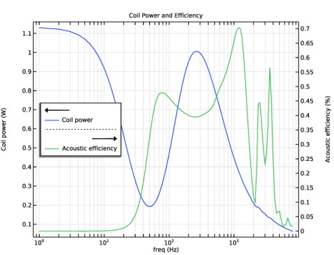
Select the Two y-axes checkbox.
|
|
4
|
|
5
|
|
6
|
|
7
|
|
8
|
|
9
|
|
10
|
|
11
|
|
12
|
|
13
|
|
1
|
|
2
|
|
3
|
|
4
|
|
5
|
Locate the Plot Settings section.
|
|
6
|
|
7
|
|
1
|
|
2
|
|
4
|
|
5
|
|
1
|
|
2
|
|
3
|
|
1
|
|
2
|
|
3
|
|
1
|
|
2
|
|
1
|
|
2
|
|
3
|
|
4
|
|
1
|
|
2
|
|
3
|
|
4
|
|
5
|
|
6
|
|
7
|
|
8
|
|
9
|
|
10
|
|
1
|
|
2
|
|
3
|
|
4
|
|
5
|
|
6
|
|
1
|
|
2
|
|
1
|
|
2
|
|
3
|
Select the Plot on secondary y-axis checkbox.
|
|
4
|
Locate the y-Axis Data section. In the table, enter the following settings:
|
|
5
|
|
6
|
|
1
|
|
2
|
Go to the Add Study window.
|
|
3
|
|
4
|
Click the Add Study button in the window toolbar.
|
|
5
|
|
1
|
In the Settings window for Frequency-Domain Perturbation, locate the Physics and Variables Selection section.
|
|
2
|
Select the Modify model configuration for study step checkbox.
|
|
3
|
In the tree, select Component 1 (comp1) > Pressure Acoustics, Frequency Domain (acpr) > Narrow Region Acoustics 1.
|
|
4
|
Click
|
|
5
|
In the tree, select Component 1 (comp1) > Pressure Acoustics, Frequency Domain (acpr) > Narrow Region Acoustics 2.
|
|
6
|
Click
|
|
7
|
|
8
|
In the Settings window for Study, type Study 3 - Complete Model, Without Narrow Region Acoustics in the Label text field.
|
|
9
|
|
10
|
|
1
|
|
2
|
|
3
|
From the Dataset list, choose Study 3 - Complete Model, Without Narrow Region Acoustics/Solution 5 (sol5).
|
|
4
|
Locate the Legends section. In the table, enter the following settings:
|
|
5
|
Locate the Coloring and Style section. Find the Line style subsection. From the Line list, choose Dotted.
|
|
1
|
|
2
|
|
3
|
|
4
|
Locate the Legends section. In the table, enter the following settings:
|
|
5
|
Locate the Coloring and Style section. Find the Line style subsection. From the Line list, choose Solid.
|
|
6
|
|
1
|
|
2
|
|
3
|
From the Dataset list, choose Study 3 - Complete Model, Without Narrow Region Acoustics/Solution 5 (sol5).
|
|
1
|
|
2
|
In the Settings window for 2D Plot Group, type Acoustic Pressure - Without Narrow Region Acoustics in the Label text field.
|
|
3
|
|
4
|
|
5
|
|
1
|
|
2
|
|
3
|
|
4
|
|
5
|
|
6
|
|
1
|
|
2
|
|
3
|
From the Dataset list, choose Study 3 - Complete Model, Without Narrow Region Acoustics/Solution 5 (sol5).
|
|
4
|
|
5
|
|
6
|
|
1
|
In the Model Builder window, right-click Acoustic Pressure - Without Narrow Region Acoustics and choose Annotation.
|
|
2
|
|
3
|
|
4
|
|
5
|
|
6
|
|
1
|
|
2
|
|
3
|
|
4
|
|
1
|
In the Model Builder window, right-click Acoustic Pressure - Without Narrow Region Acoustics and choose Line.
|
|
2
|
|
3
|
|
4
|
|
5
|
|
6
|
|
7
|
|
8
|
|
9
|
|
1
|
|
2
|
Go to the Add Study window.
|
|
3
|
Find the Physics interfaces in study subsection. In the table, clear the Solve checkboxes for Magnetic Fields (mf) and Pressure Acoustics, Frequency Domain (acpr).
|
|
4
|
Find the Multiphysics couplings in study subsection. In the table, clear the Solve checkboxes for Acoustic–Structure Boundary 1 (asb1) and Magnetomechanics, Solid 1 (mmcpl1).
|
|
5
|
|
6
|
Click the Add Study button in the window toolbar.
|
|
7
|
|
1
|
|
2
|
|
3
|
|
4
|
|
5
|
|
1
|
|
2
|
|
3
|
|
4
|
|
1
|
|
1
|
|
2
|
|
1
|
|
2
|
|
3
|
|
4
|
Click to expand the Layers section. In the table, enter the following settings:
|
|
1
|
|
2
|
|
3
|
|
4
|
|
5
|
|
6
|
Locate the Layers section. In the table, enter the following settings:
|
|
1
|
|
2
|
On the object c2, select Boundaries 2–4 only.
|
|
1
|
|
2
|
|
3
|
|
4
|
|
5
|
|
6
|
|
1
|
|
2
|
Select the object c1 only.
|
|
3
|
|
4
|
|
5
|
Select the object r1 only.
|
|
1
|
|
2
|
|
3
|
|
4
|
|
5
|
|
6
|
|
1
|
|
2
|
|
3
|
|
4
|
|
5
|
|
6
|
|
1
|
|
2
|
|
3
|
|
4
|
|
5
|
|
6
|
|
1
|
|
2
|
|
3
|
|
4
|
|
5
|
|
6
|
|
1
|
|
2
|
|
3
|
|
4
|
|
5
|
|
1
|
|
2
|
Select the object r2 only.
|
|
3
|
|
4
|
|
5
|
|
1
|
|
2
|
|
3
|
|
4
|
|
5
|
|
6
|
|
7
|
Click to expand the Layers section. In the table, enter the following settings:
|
|
8
|
Clear the Layers on bottom checkbox.
|
|
9
|
Select the Layers on top checkbox.
|
|
1
|
|
2
|
|
3
|
|
4
|
|
5
|
|
6
|
|
1
|
|
2
|
|
3
|
|
4
|
In the r text field, type 18.4[mm] 23[mm] 26[mm] 26[mm] 32[mm] 32[mm] 38[mm] 38[mm] 44[mm] 44[mm] 50[mm] 50[mm] 56[mm] 56[mm] 59[mm] 66[mm] 66[mm] 59[mm] 56[mm] 56[mm] 50[mm] 50[mm] 44[mm] 44[mm] 38[mm] 38[mm] 32[mm] 32[mm] 26[mm] 26[mm] 23[mm] 18.4[mm].
|
|
5
|
In the z text field, type -44.1[mm] -44.1[mm] -42.1[mm] -42.1[mm] -46.1[mm] -46.1[mm] -42.1[mm] -42.1[mm] -46.1[mm] -46.1[mm] -42.1[mm] -42.1[mm] -46.1[mm] -46.1[mm] -44.1[mm] -44.1[mm] -44.5[mm] -44.5[mm] -46.5[mm] -46.5[mm] -42.5[mm] -42.5[mm] -46.5[mm] -46.5[mm] -42.5[mm] -42.5[mm] -46.5[mm] -46.5[mm] -42.5[mm] -42.5[mm] -44.5[mm] -44.5[mm].
|
|
1
|
|
2
|
|
3
|
|
4
|
|
5
|
|
1
|
|
2
|
|
3
|
|
4
|
|
5
|
|
6
|
|
7
|
|
8
|
|
1
|
|
2
|
|
3
|
|
4
|
|
5
|
|
6
|
|
7
|
|
8
|
|
1
|
|
2
|
|
3
|
|
4
|
|
5
|
|
6
|
|
7
|
|
8
|
|
1
|
|
2
|
|
3
|
|
4
|
|
5
|
|
6
|
|
7
|
|
8
|
|
1
|
|
2
|
On the object dif2, select Points 5–8 only.
|
|
3
|
|
4
|
|
1
|
|
2
|
|
3
|
|
4
|
|
5
|
|
6
|
|
7
|