| 
|
|
|
|




|
•
|
As a general rule of thumb, at least five quadratic elements should be used to resolve each wavelength. Therefore, the maximum mesh element size is set to 1/5 of the shortest wavelengths present, c_air/fmax. This mesh size is artificially refined to increase the running time.
|
|
•
|
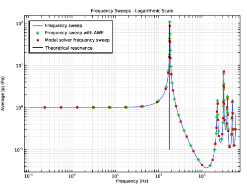
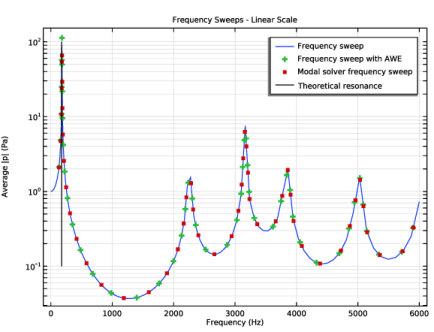
When several resonance frequencies are present, the default parameters for the AWE option may use some tuning, for example, using an adequate Absolute tolerance value (see under the >AWE Solver 1 node). In this model, the default value of 0.001 is used and gives reasonable results (when compared to the other methods). Lowering the value to 0.0001 will improve the high frequency results slightly (see the linear scale plot). Other settings are in general less important, like changing the number of points to linearize about (Evaluation points), changing the number of terms in the Taylor expansion about each point (Expansion size), or changing from Padé to Taylor expansion of the approximating solution (Expansion type). In the current setup, we chose a relatively high upper frequency bound so about 10 resonance frequencies are present in the sweep. Had the upper frequency limit been lowered so only the first resonance was included (for instance, by setting fmax = 100 Hz), then the default relative AWE tolerance would have sufficed. Note that if either end of the frequency range is close to a resonance, the AWE solver can become unreliable.
|
|
•
|
The linper operator informs the solver that the term in the expression is a perturbation (a source term) that must be included in the linearized problem. The modal solver will only use the pressure under the linper operator as a source, while the other solvers will ignore this perturbation term.
|
|
•
|
To obtain good results with the Modal solver up to fmax, we must set the upper limit in its eigenfrequency search to 1.5*fmax to capture modes that may have an influence on the highest part of the frequency of interest. Using only fmax as the upper limit results in poorer estimates of the solution at higher frequencies.
|
|
•
|
Not all resonance peaks may be captured with the current frequency resolution used in this tutorial, because it gets coarser as the frequency increases. For example, there is a narrow resonance peak at about 4.9 kHz that lies within the interval [fmin, fmax], but not visible in Figure 4 or Figure 5. However, it is detected by the Eigenvalue solver used in the last study. Another indication is the warning message produced by the Adaptive Frequency Sweep with AWE solver which suggests that the frequency sampling should be refined.
|
|
•
|
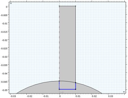
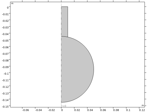
Finally, note that we define the model in terms of geometric parameters (a, L, and R). This makes it easy to quickly include parametric sweeps in the geometry, which, for instance, could be used to tune the lowest eigenfrequency.
|
|
1
|
|
2
|
In the Select Physics tree, select Acoustics > Pressure Acoustics > Pressure Acoustics, Frequency Domain (acpr).
|
|
3
|
Click Add.
|
|
4
|
Click
 Study. Study. |
|
5
|
|
6
|
Click
 Done. Done. |
|
1
|
|
2
|
|
3
|
Click
 Load from File. Load from File. |
|
4
|
Browse to the model’s Application Libraries folder and double-click the file helmholtz_resonator_solvers_parameters.txt.
|
|
1
|
|
2
|
|
3
|
|
4
|
|
5
|
|
1
|
|
2
|
|
3
|
|
4
|
|
1
|
|
2
|
Click in the Graphics window and then press Ctrl+A to select both objects.
|
|
1
|
|
2
|
|
3
|
|
4
|
|
5
|
|
1
|
In the Model Builder window, under Component 1 (comp1) right-click Materials and choose Blank Material.
|
|
2
|
|
3
|
Locate the Material Contents section. In the table, enter the following settings:
|
|
1
|
|
1
|
|
1
|
|
3
|
|
4
|
|
1
|
|
2
|
In the Settings window for AWE Expression, locate the Asymptotic Waveform Evaluation Expression section.
|
|
3
|
|
1
|
|
2
|
|
3
|
|
4
|
|
5
|
|
6
|
|
7
|
Click
 Build All. Build All. |
|
1
|
|
2
|
|
3
|
|
1
|
|
2
|
|
3
|
In the Frequencies text field, type 10^{range(log10(fmin),(log10(fmax)-(log10(fmin)))/499,log10(fmax))}.
|
|
4
|
|
1
|
|
2
|
Go to the Add Study window.
|
|
3
|
Find the Studies subsection. In the Select Study tree, select Preset Studies for Selected Physics Interfaces > Adaptive Frequency Sweep.
|
|
4
|
Click the Add Study button in the window toolbar.
|
|
5
|
|
1
|
|
2
|
In the Frequencies text field, type 10^{range(log10(fmin),(log10(fmax)-(log10(fmin)))/499,log10(fmax))}.
|
|
3
|
|
4
|
|
5
|
|
6
|
|
7
|
Clear the Generate default plots checkbox.
|
|
8
|
|
9
|
|
1
|
|
2
|
Go to the Add Study window.
|
|
3
|
Find the Studies subsection. In the Select Study tree, select Preset Studies for Selected Physics Interfaces > Frequency Domain, Modal.
|
|
4
|
Click the Add Study button in the window toolbar.
|
|
5
|
|
1
|
|
2
|
Clear the Generate default plots checkbox.
|
|
3
|
|
1
|
In the Model Builder window, under Study 3 - Modal solver frequency sweep click Step 1: Eigenfrequency.
|
|
2
|
|
3
|
|
4
|
Find the Rectangle search region subsection. In the Largest real part (Eigenfrequency) text field, type 1.5*fmax.
|
|
1
|
|
2
|
|
3
|
In the Frequencies text field, type 10^{range(log10(fmin),(log10(fmax)-(log10(fmin)))/499,log10(fmax))}.
|
|
4
|
|
1
|
|
2
|
In the Settings window for 1D Plot Group, type Frequency Sweeps - Logarithmic Scale in the Label text field.
|
|
3
|
|
4
|
Locate the Plot Settings section.
|
|
5
|
|
6
|
|
7
|
|
8
|
Select the y-axis log scale checkbox.
|
|
9
|
|
1
|
|
2
|
|
3
|
|
4
|
|
6
|
|
7
|
|
8
|
|
9
|
|
10
|
|
1
|
|
2
|
|
3
|
|
4
|
Click to expand the Coloring and Style section. Find the Line style subsection. From the Line list, choose None.
|
|
5
|
|
6
|
|
7
|
|
8
|
Locate the Legends section. In the table, enter the following settings:
|
|
1
|
|
2
|
|
3
|
|
4
|
Locate the Coloring and Style section. Find the Line markers subsection. From the Marker list, choose Point.
|
|
5
|
Locate the Legends section. In the table, enter the following settings:
|
|
1
|
|
2
|
|
3
|
|
4
|
Locate the x-Coordinates section. In the table, enter the following settings:
|
|
5
|
Locate the y-Coordinates section. In the table, enter the following settings:
|
|
6
|
|
7
|
|
8
|
|
10
|
|
1
|
|
2
|
|
3
|
Clear the x-axis log scale checkbox.
|
|
4
|
|
5
|
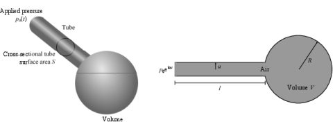
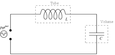
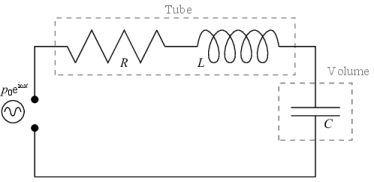
 and the tube is cylindrical so
  illustrating agreement between all solvers and the theory for the first eigenfrequency and also illustrating agreement between all solvers for the higher frequencies.