|
|
|

|
•
|
|
•
|


|
1
|
|
2
|
|
3
|
Click Add.
|
|
4
|
|
5
|
Click Add.
|
|
6
|
In the Select Physics tree, select Mathematics > ODE and DAE Interfaces > Boundary ODEs and DAEs (bode).
|
|
7
|
Click Add.
|
|
8
|
Click
|
|
9
|
|
10
|
Click
|
|
1
|
|
2
|
|
3
|
Locate the Parameters section. In the table, enter the following settings:
|
|
1
|
|
2
|
|
3
|
Locate the Parameters section. In the table, enter the following settings:
|
|
1
|
|
2
|
|
3
|
Locate the Parameters section. In the table, enter the following settings:
|
|
1
|
|
2
|
|
3
|
Locate the Parameters section. In the table, enter the following settings:
|
|
1
|
|
2
|
|
3
|
|
4
|
|
5
|
|
6
|
Locate the Selections of Resulting Entities section. Select the Resulting objects selection checkbox.
|
|
1
|
|
2
|
|
3
|
|
4
|
|
1
|
|
2
|
|
3
|
|
4
|
Locate the Selections of Resulting Entities section. Select the Resulting objects selection checkbox.
|
|
1
|
|
2
|
|
3
|
|
1
|
|
2
|
|
3
|
|
4
|
Locate the Coordinates section. In the table, enter the following settings:
|
|
5
|
Locate the Selections of Resulting Entities section. Select the Resulting objects selection checkbox.
|
|
6
|
|
1
|
|
2
|
|
3
|
|
4
|
|
5
|
|
6
|
Locate the Spine Curve section. Click to select the
|
|
7
|
|
8
|
On the object wp2, select Edges 1–4 only.
|
|
9
|
Locate the Input Object Handling section. Select the Include all inputs in Form Union/Assembly checkbox.
|
|
10
|
Locate the Motion of Cross Section section. Find the Additional twisting and scaling subsection. In the Scale factor text field, type (1-(r_hillock-r_AIS)/r_hillock*s).
|
|
11
|
Locate the Selections of Resulting Entities section. Select the Resulting objects selection checkbox.
|
|
1
|
|
2
|
|
3
|
Locate the Cross Section section. Click to select the
|
|
4
|
In the tree, select wp1.
|
|
5
|
|
6
|
On the object swe1, select Boundary 4 only.
|
|
7
|
Locate the Spine Curve section. Click to select the
|
|
8
|
In the tree, select wp2.
|
|
9
|
|
10
|
On the object wp2, select Edge 5 only.
|
|
11
|
Locate the Motion of Cross Section section. Find the Additional twisting and scaling subsection. In the Scale factor text field, type (1-(r_AIS-r_axon)/r_AIS*s).
|
|
12
|
Click
|
|
1
|
|
2
|
|
3
|
|
4
|
On the object wp2, select Point 6 only.
|
|
1
|
|
2
|
|
3
|
|
4
|
Locate the Coordinates section. In the table, enter the following settings:
|
|
5
|
Locate the Selections of Resulting Entities section. Select the Resulting objects selection checkbox.
|
|
6
|
|
1
|
In the Model Builder window, under Component 1 (comp1) > Geometry 1 right-click AIS (swe2) and choose Duplicate.
|
|
2
|
|
3
|
Locate the Cross Section section. Click to select the
|
|
4
|
In the tree, select swe1.
|
|
5
|
|
6
|
On the object swe2, select Boundary 4 only.
|
|
7
|
Locate the Spine Curve section. Click to select the
|
|
8
|
In the tree, select wp2.
|
|
9
|
|
10
|
On the object wp3, select Edge 1 only.
|
|
11
|
Locate the Motion of Cross Section section. Find the Additional twisting and scaling subsection. In the Scale factor text field, type 1.
|
|
12
|
Click
|
|
1
|
|
2
|
|
3
|
|
4
|
|
1
|
|
2
|
|
3
|
|
4
|
Locate the Selections of Resulting Entities section. Select the Resulting objects selection checkbox.
|
|
1
|
|
2
|
|
4
|
Locate the Selections of Resulting Entities section. Select the Resulting objects selection checkbox.
|
|
5
|
|
1
|
In the Model Builder window, under Component 1 (comp1) > Geometry 1 right-click Axon (swe3) and choose Duplicate.
|
|
2
|
|
3
|
|
4
|
Locate the Cross Section section. Click to select the
|
|
5
|
In the tree, select swe2.
|
|
6
|
|
7
|
|
8
|
Locate the Spine Curve section. Click to select the
|
|
9
|
In the tree, select wp3.
|
|
10
|
|
11
|
On the object wp5, select Edge 1 only.
|
|
12
|
Locate the Motion of Cross Section section. Find the Additional twisting and scaling subsection. In the Scale factor text field, type (1-(r_dendrite_ini-r_dendrite_fin)/r_dendrite_ini*s).
|
|
13
|
Click
|
|
1
|
|
2
|
|
3
|
|
4
|
Select the Keep input objects checkbox.
|
|
5
|
|
6
|
|
1
|
|
2
|
|
3
|
|
4
|
|
5
|
|
6
|
|
7
|
|
8
|
|
9
|
Click
|
|
1
|
|
2
|
|
3
|
|
4
|
|
5
|
On the object blk1, select Point 1 only.
|
|
6
|
Locate the Selections of Resulting Entities section. Find the Selections from plane geometry subsection. Select the Show in physics checkbox.
|
|
1
|
|
2
|
|
3
|
|
4
|
|
5
|
|
1
|
|
2
|
Select the object c1 only.
|
|
3
|
|
4
|
|
5
|
|
6
|
|
7
|
|
8
|
Locate the Selections of Resulting Entities section. Select the Resulting objects selection checkbox.
|
|
1
|
|
2
|
|
3
|
|
4
|
|
5
|
|
6
|
|
1
|
|
2
|
|
3
|
|
4
|
|
5
|
|
6
|
|
7
|
Click
|
|
1
|
In the Model Builder window, right-click Geometry 1 and choose Booleans and Partitions > Difference.
|
|
2
|
|
3
|
|
4
|
|
5
|
|
6
|
Select the Keep objects to subtract checkbox.
|
|
1
|
|
2
|
On the object wp1, select Boundary 1 only.
|
|
1
|
|
2
|
|
3
|
|
4
|
On the object wp2, select Edges 1–5 only.
|
|
5
|
On the object wp3, select Edge 1 only.
|
|
6
|
Click
|
|
7
|
|
8
|
Click
|
|
1
|
Go to the Cleanup Wizard window.
|
|
2
|
Click the Manual button.
|
|
3
|
|
4
|
Click the Apply button in the window toolbar.
|
|
5
|
Click the Apply button in the window toolbar.
|
|
6
|
Click the Done button in the window toolbar.
|
|
1
|
|
2
|
|
3
|
|
4
|
On the object aigv2, select Boundary 1 only.
|
|
5
|
On the object aigv2, select Boundary 4 only.
|
|
6
|
On the object aigv2, select Boundary 2 only.
|
|
7
|
|
1
|
|
2
|
|
3
|
|
4
|
|
5
|
Click OK.
|
|
1
|
|
2
|
|
3
|
|
4
|
|
5
|
Click OK.
|
|
1
|
|
2
|
|
3
|
|
4
|
On the object aigv2, select Boundaries 7, 113, and 189 only.
|
|
5
|
|
1
|
|
2
|
|
3
|
|
4
|
|
5
|
|
6
|
Click OK.
|
|
7
|
|
8
|
|
9
|
|
10
|
Click OK.
|
|
1
|
|
2
|
|
3
|
|
4
|
|
5
|
Click OK.
|
|
1
|
|
2
|
|
3
|
|
4
|
|
5
|
|
6
|
|
7
|
Locate the Variables section. In the table, enter the following settings:
|
|
1
|
|
2
|
|
3
|
|
4
|
|
5
|
|
6
|
Locate the Variables section. In the table, enter the following settings:
|
|
1
|
|
2
|
|
3
|
|
4
|
|
5
|
|
6
|
Locate the Variables section. In the table, enter the following settings:
|
|
1
|
|
2
|
|
3
|
|
4
|
|
5
|
|
6
|
Locate the Variables section. In the table, enter the following settings:
|
|
1
|
|
2
|
|
3
|
|
4
|
|
5
|
|
6
|
Locate the Variables section. In the table, enter the following settings:
|
|
1
|
|
2
|
|
3
|
|
4
|
|
5
|
|
6
|
Locate the Variables section. In the table, enter the following settings:
|
|
1
|
|
2
|
|
3
|
|
4
|
Locate the Definition section. In the Expression text field, type -0.09575*(Vmembrane/1[mV]+37)/(exp(-0.1*(Vmembrane/1[mV]+37))-1).
|
|
5
|
|
6
|
Locate the Units section. In the table, enter the following settings:
|
|
7
|
|
1
|
|
2
|
|
3
|
|
4
|
Locate the Definition section. In the Expression text field, type 1.915*exp(-(Vmembrane/1[mV]+47)/80).
|
|
1
|
In the Model Builder window, under Component 1 (comp1) > Definitions, Ctrl-click to select alpha_n (alpha_n) and beta_n (beta_n).
|
|
2
|
Right-click and choose Duplicate.
|
|
1
|
|
2
|
|
3
|
Locate the Definition section. In the Expression text field, type -2.725*(Vmembrane/1[mV]+35)/(exp(-0.1*(Vmembrane/1[mV]+35))-1).
|
|
1
|
|
2
|
|
3
|
|
4
|
Locate the Definition section. In the Expression text field, type 90.83*exp(-(Vmembrane/1[mV]+60)/20).
|
|
1
|
In the Model Builder window, under Component 1 (comp1) > Definitions right-click alpha_n (alpha_n) and choose Duplicate.
|
|
2
|
|
3
|
|
4
|
Locate the Definition section. In the Expression text field, type 1.817*exp(-(Vmembrane/1[mV]+52)/20).
|
|
1
|
In the Model Builder window, under Component 1 (comp1) > Definitions right-click beta_n (beta_n) and choose Duplicate.
|
|
2
|
|
3
|
|
4
|
Locate the Definition section. In the Expression text field, type 27.25/(exp(-0.1*(Vmembrane/1[mV]+22))+1).
|
|
1
|
In the Model Builder window, under Component 1 (comp1) > Definitions right-click alpha_n (alpha_n) and choose Duplicate.
|
|
2
|
|
3
|
|
4
|
Locate the Definition section. In the Expression text field, type alpha_n(Vmembrane)/(alpha_n(Vmembrane)+beta_n(Vmembrane)).
|
|
5
|
|
1
|
|
2
|
|
3
|
|
4
|
Locate the Definition section. In the Expression text field, type alpha_m(Vmembrane)/(alpha_m(Vmembrane)+beta_m(Vmembrane)).
|
|
1
|
|
2
|
|
3
|
|
4
|
Locate the Definition section. In the Expression text field, type alpha_h(Vmembrane)/(alpha_h(Vmembrane)+beta_h(Vmembrane)).
|
|
1
|
In the Model Builder window, under Component 1 (comp1) > Definitions, Ctrl-click to select alpha_n (alpha_n), beta_n (beta_n), alpha_m (alpha_m), beta_m (beta_m), alpha_h (alpha_h), beta_h (beta_h), n_inf (n_inf), m_inf (m_inf), and h_inf (h_inf).
|
|
2
|
Right-click and choose Group.
|
|
1
|
|
2
|
|
3
|
|
4
|
|
5
|
|
1
|
|
2
|
|
3
|
Click
|
|
4
|
Click
|
|
5
|
|
6
|
|
7
|
|
8
|
|
1
|
|
2
|
|
3
|
|
4
|
|
1
|
|
2
|
|
3
|
|
4
|
|
1
|
|
2
|
|
3
|
|
4
|
|
1
|
|
2
|
|
3
|
|
4
|
|
1
|
|
2
|
|
3
|
|
4
|
|
1
|
|
2
|
Go to the Add Material window.
|
|
1
|
In the Model Builder window, under Component 1 (comp1) right-click Materials and choose Blank Material.
|
|
2
|
|
3
|
|
4
|
|
6
|
Locate the Material Contents section. In the table, enter the following settings:
|
|
1
|
|
2
|
|
3
|
Locate the Material Contents section. In the table, enter the following settings:
|
|
4
|
|
5
|
|
7
|
|
1
|
|
2
|
|
3
|
|
4
|
Click to expand the Dependent Variables section. In the Electric potential (V) text field, type Vout.
|
|
5
|
|
1
|
|
1
|
|
2
|
|
3
|
|
4
|
|
1
|
|
2
|
|
3
|
|
1
|
|
2
|
|
3
|
|
4
|
|
1
|
|
2
|
|
3
|
|
1
|
|
2
|
|
3
|
|
4
|
|
1
|
|
2
|
|
3
|
|
4
|
|
1
|
|
2
|
|
3
|
|
4
|
|
5
|
|
6
|
Click to expand the Dependent Variables section. In the Dependent variables (1) table, enter the following settings:
|
|
7
|
Click
|
|
8
|
In the Dependent variables (1) table, enter the following settings:
|
|
9
|
Click
|
|
10
|
In the Dependent variables (1) table, enter the following settings:
|
|
1
|
In the Model Builder window, under Component 1 (comp1) > Boundary ODEs and DAEs (bode) click Distributed ODE 1.
|
|
2
|
|
3
|
|
4
|
|
5
|
|
1
|
|
2
|
|
3
|
|
4
|
|
5
|
|
1
|
|
2
|
|
3
|
|
4
|
|
1
|
|
2
|
|
3
|
|
1
|
In the Model Builder window, under Component 1 (comp1) > Mesh 1, Ctrl-click to select Size 1 and Size 2.
|
|
2
|
Right-click and choose Delete.
|
|
1
|
|
2
|
|
3
|
|
4
|
|
6
|
|
7
|
Locate the Element Size Parameters section.
|
|
8
|
|
9
|
|
10
|
|
11
|
|
12
|
|
13
|
|
14
|
|
18
|
|
1
|
|
2
|
|
3
|
Clear the Generate default plots checkbox.
|
|
1
|
|
2
|
|
3
|
|
4
|
|
1
|
|
2
|
|
3
|
In the Model Builder window, under Study 1 > Solver Configurations > Solution 1 (sol1) click Time-Dependent Solver 1.
|
|
4
|
|
5
|
|
6
|
Right-click Study 1 > Solver Configurations > Solution 1 (sol1) > Time-Dependent Solver 1 and choose Fully Coupled.
|
|
7
|
|
1
|
|
2
|
|
3
|
|
4
|
|
1
|
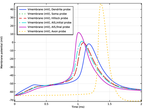
In the Model Builder window, expand the Results > Probe Plot Group 1 node, then click Probe Plot Group 1.
|
|
2
|
In the Settings window for 1D Plot Group, type Action Potential Generation and Propagation in the Label text field.
|
|
3
|
Locate the Plot Settings section.
|
|
4
|
|
5
|
|
1
|
|
2
|
|
3
|
|
4
|
|
5
|
|
1
|
|
2
|
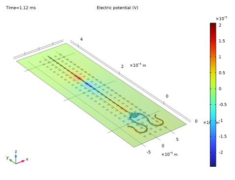
In the Settings window for 3D Plot Group, type Electric Potential at MEA Plane in the Label text field.
|
|
3
|
|
4
|
|
1
|
|
2
|
|
3
|
|
4
|
|
1
|
|
2
|
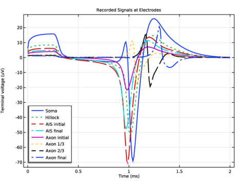
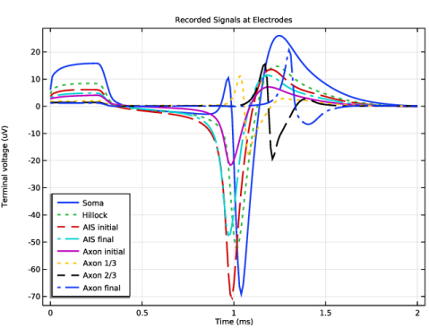
In the Settings window for 1D Plot Group, type Recorded Signals at Electrodes in the Label text field.
|
|
3
|
|
4
|
|
1
|
|
2
|
|
3
|
|
4
|
|
5
|
Locate the y-Axis Data section. In the table, enter the following settings:
|
|
6
|
|
8
|
|
9
|