PDF

Magnetic Damping of Vibrating Conducting Solids
Introduction
When a conductive solid material moves through a static magnetic field, an eddy current density is induced. That induced eddy current density interacts with the static magnetic field, and the result is a Lorentz force acting on the solid that counteracts the motion. Therefore, a conducting solid that is oscillating in a static magnetic field experiences structural damping.
This example computes the damping effect in two different ways. First, by harmonically exciting a cantilever beam across a range of frequencies and placing it in a strong magnetic field. The same effect is then computed in a full transient study when the beam instead experiences a sudden applied load. The approach presented here assumes that the relative magnitudes of the structural displacements are small, that the material has isotropic and linear properties, and that the damping Lorentz force can be computed from the static magnetic field and the motion induced AC eddy current density. Second-order effects arising from the AC magnetic field generated by the eddy currents are not included in the computation. The AC magnetic field is also computed and found to be 2–3 orders of magnitude smaller than the DC magnetic field.
Figure 1: A vibrating beam next to a current-carrying wire experiences magnetic damping.
Model Definition
For a solid material experiencing a time-harmonic forced excitation, the displacement field is of the form
,
which can also be written in the frequency domain as a phasor:
Thus, the velocity field is given by
In the transient study, the displacement field is not necessarily an exact sine wave. However, as can be seen in Figure 5, it behaves similarly. In that case, it is already slightly damped even without the addition of the magnetic field, as it approaches its equilibrium position.
Next, consider the effect of a spatially nonuniform, but static, magnetic flux density BDC(r). Under the assumption that the local displacements are small enough for each moving point in the solid to only see the magnetic flux density in the undeformed state, the velocity induced current density is given by
where σ is the material conductivity. The resulting total AC current density is different, as the metallic cantilever beam is inductive and therefore exhibits a skin effect. Thus, a second, magnetodynamic, problem has to be solved in order to compute the AC current density. The body forces experienced by a current-carrying domain moving through a magnetic field are then given by the cross product between the induced AC current density and the static magnetic flux density:
These body forces are then applied to the structural mechanics problem and act as a damping force on the system.
The application contains two different studies, both of which first compute the static magnetic field due to a current-carrying wire which is next to an aluminum beam. In the first case, the second step is set as a Frequency Domain Perturbation study. There, the beam experiences a forced harmonic vibration and the resulting mechanical beam displacement field and AC current density are computed, yielding also the damping electromagnetic force. In the second case, the second step is instead set as a Time Dependent study, where the full transient solution is found. A constant boundary load is applied to the end of the beam instead of the harmonic perturbation in the previous case. However, since that load is applied suddenly at the start of the study instead of ramping up slowly, it will still cause the beam to oscillate.
In both cases, the strength of the magnetic field is then varied through a Parametric Sweep, and the effect of the magnetic damping on the response of the system can be observed and compared between the two approaches.
Results and Discussion
Figure 2 shows the magnetic flux density computed for the structure at rest. Figure 3 displays the magnitude of the displacement of the tip of the beam versus excitation frequency for two different magnetic field intensities for the frequency-domain structural dynamics problem. The magnetic field provides significant additional damping. Figure 4 shows a snapshot of the induced eddy current distribution in the beam. Figure 5 shows how the displacement of the tip of the beam varies with time in the full time dependent model. There, the effects of the magnetic damping become even more apparent. The amplitude of the oscillations decreases much quicker with time when a current passes through the wire, compared to the case where there is no current. It is also interesting to compare the results in that plot with the results in the corresponding plot from the frequency domain, shown in Figure 3.
Figure 2: The magnetic field around a current-carrying wire.
Figure 3: Displacement of the tip of the beam versus excitation frequency for differing values of the current through the wire.
Figure 4: The AC current distribution.
Figure 5: Displacement of the tip of the beam as a function of time, for different values of the current through the wire.
Notes About the COMSOL Implementation
Solve this application with two physics interfaces: the Magnetic Fields and Solid Mechanics interfaces. Use a Stationary study for the first Magnetic Fields interface and either a Frequency Domain Perturbation study or a Time Dependent study for the Magnetic Fields and Solid Mechanics interfaces. The coupling between the two interfaces is automatically considered by using the Magnetomechanics multiphysics coupling feature.
Application Library path: ACDC_Module/Electromagnetics_and_Mechanics/magnetic_damping
Modeling Instructions
From the File menu, choose New.
New
In the New window, click  Model Wizard.
Model Wizard
1
In the Model Wizard window, click  3D.
2
In the Select Physics tree, select AC/DC > Electromagnetic Fields > Magnetic Fields (mf).
3
Click Add.
4
In the Select Physics tree, select Structural Mechanics > Solid Mechanics (solid).
5
Click Add.
6
Click  Study.
7
In the Select Study tree, select Empty Study.
8
Global Definitions
Parameters 1
1
In the Model Builder window, under Global Definitions click Parameters 1.
2
In the Settings window for Parameters, locate the Parameters section.
3
The Applied current will be used as a sweep parameter.
Geometry 1
1
In the Model Builder window, under Component 1 (comp1) click Geometry 1.
2
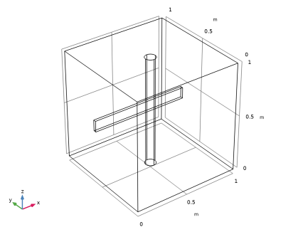
In the Geometry toolbar, click Block to create a block for the simulation domain. Leave the default block size.
3
In the Geometry toolbar, click Block again to create a block for the cantilever beam.
Cantilever Beam
1
In the Model Builder window, under Component 1 (comp1) > Geometry 1 click Block 2 (blk2).
2
In the Settings window for Block, type Cantilever Beam in the Label text field.
3
Locate the Size and Shape section. In the Width text field, type 0.9.
4
In the Depth text field, type 0.025.
5
In the Height text field, type 0.1.
6
Locate the Position section. In the y text field, type 0.575.
7
In the z text field, type 0.45.
8
Locate the Selections of Resulting Entities section. Select the Resulting objects selection checkbox.
Finally, add a cylinder for the wire generating the static magnetic field.
Cylindrical Coil
1
In the Geometry toolbar, click  Cylinder.
2
In the Settings window for Cylinder, type Cylindrical Coil in the Label text field.
3
Locate the Size and Shape section. In the Radius text field, type r0.
4
Locate the Position section. In the x text field, type 0.5.
5
In the y text field, type 0.5.
6
Locate the Selections of Resulting Entities section. Select the Resulting objects selection checkbox.
7
Click  Build All Objects.
8
Click the  Wireframe Rendering button in the Graphics toolbar.
Add variables for the induced current density and body force on the cantilever beam.
Magnetic Fields (mf)
Ampère’s Law in Solids 1
1
In the Physics toolbar, click  Domains and choose Ampère’s Law in Solids.
2
In the Settings window for Ampère’s Law in Solids, locate the Domain Selection section.
3
From the Selection list, choose Cantilever Beam.
Domain Coil 1
1
In the Physics toolbar, click  Domains and choose Domain Coil.
2
In the Settings window for Domain Coil, locate the Domain Selection section.
3
From the Selection list, choose Cylindrical Coil.
4
Locate the Coil section. From the Conductor model list, choose Homogenized multiturn.
5
From the Coil type list, choose Linear.
6
In the Icoil text field, type a_c.
7
Locate the Homogenized Conductor section. In the N text field, type 1.
8
From the Coil wire cross-section area list, choose From diameter.
9
In the d text field, type 2*r0.
Coil Geometry 1
1
In the Model Builder window, click Coil Geometry 1.
2
Free Space 1
The Free Space feature adds a small electric conductivity to the surrounding volume for numerical stabilization.
1
In the Model Builder window, under Component 1 (comp1) > Magnetic Fields (mf) click Free Space 1.
2
In the Settings window for Free Space, locate the Stabilization section.
3
From the σstab list, choose User defined. In the associated text field, type 10[S/m].
Solid Mechanics (solid)
The Solid Mechanics interface is active only on the cantilever beam.
1
In the Model Builder window, under Component 1 (comp1) click Solid Mechanics (solid).
2
In the Settings window for Solid Mechanics, locate the Domain Selection section.
3
From the Selection list, choose Cantilever Beam.
Linear Elastic Material 1
Add a damping factor on Linear Elastic Material Model 1.
1
In the Model Builder window, under Component 1 (comp1) > Solid Mechanics (solid) click Linear Elastic Material 1.
Damping 1
1
In the Physics toolbar, click  Attributes and choose Damping.
2
In the Settings window for Damping, locate the Damping Settings section.
3
From the Damping type list, choose Isotropic loss factor.
4
From the ηs list, choose User defined. In the associated text field, type 0.1.
Fixed Constraint 1
1
In the Physics toolbar, click  Boundaries and choose Fixed Constraint.
2
Harmonic Boundary Load for Frequency-Domain Vibration Analysis
1
In the Physics toolbar, click  Boundaries and choose Boundary Load.
2
3
In the Settings window for Boundary Load, type Harmonic Boundary Load for Frequency-Domain Vibration Analysis in the Label text field.
4
Locate the Force section. Specify the fA vector as
5
Right-click Harmonic Boundary Load for Frequency-Domain Vibration Analysis and choose Harmonic Perturbation.
Boundary Load for Time-Dependent Analysis
1
In the Physics toolbar, click  Boundaries and choose Boundary Load.
2
3
In the Settings window for Boundary Load, type Boundary Load for Time-Dependent Analysis in the Label text field.
4
Locate the Force section. Specify the fA vector as
Add Material
1
In the Materials toolbar, click  Add Material to open the Add Material window.
2
Go to the Add Material window.
3
In the tree, select Built-in > Aluminum.
4
Click the Add to Component button in the window toolbar.
5
In the Materials toolbar, click  Add Material to close the Add Material window.
Materials
Aluminum (mat1)
1
In the Settings window for Material, locate the Geometric Entity Selection section.
2
From the Selection list, choose Cantilever Beam.
Multiphysics
Magnetomechanics, Solid 1 (mmcpl1)
1
In the Physics toolbar, click  Multiphysics Couplings and choose Domain > Magnetomechanics, Solid.
2
In the Settings window for Magnetomechanics, Solid, locate the Lorentz Coupling section.
3
Select the Only use Lorentz force checkbox.
Mesh 1
1
In the Model Builder window, under Component 1 (comp1) click Mesh 1.
2
In the Settings window for Mesh, locate the Physics-Controlled Mesh section.
3
From the Element size list, choose Coarser.
Frequency-Domain Vibration Analysis
1
In the Model Builder window, click Study 1.
2
In the Settings window for Study, type Frequency-Domain Vibration Analysis in the Label text field.
Parametric Sweep
1
In the Study toolbar, click  Parametric Sweep.
2
In the Settings window for Parametric Sweep, locate the Study Settings section.
3
4
Step 1: Stationary
1
In the Study toolbar, click  Stationary.
2
In the Settings window for Stationary, locate the Physics and Variables Selection section.
3
In the Solve for column of the table, under Component 1 (comp1), clear the checkbox for Solid Mechanics (solid).
4
In the Solve for column of the table, under Component 1 (comp1) > Multiphysics, clear the checkbox for Magnetomechanics, Solid 1 (mmcpl1).
Step 2: Frequency-Domain Perturbation
1
In the Study toolbar, click  More Study Steps and choose Frequency Domain > Frequency-Domain Perturbation.
2
In the Settings window for Frequency-Domain Perturbation, locate the Study Settings section.
3
In the Frequencies text field, type range(5,0.5,50).
4
Locate the Physics and Variables Selection section. Select the Modify model configuration for study step checkbox.
5
In the tree, select Component 1 (comp1) > Solid Mechanics (solid) > Boundary Load for Time-Dependent Analysis.
6
Solution 1 (sol1)
1
In the Study toolbar, click  Show Default Solver.
Some adjustments to the default solver settings will improve the performance.
2
In the Model Builder window, expand the Solution 1 (sol1) node.
3
In the Model Builder window, expand the Frequency-Domain Vibration Analysis > Solver Configurations > Solution 1 (sol1) > Stationary Solver 2 node, then click Fully Coupled 1.
4
In the Settings window for Fully Coupled, locate the General section.
5
From the Linear solver list, choose Direct.
6
In the Study toolbar, click  Compute.
Results
DC Magnetic Flux Density Norm
The first default plot group shows the magnetic field around a current carrying wire; compare with Figure 2. Give it a more descriptive name.
1
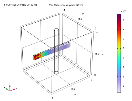
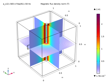
In the Settings window for 3D Plot Group, type DC Magnetic Flux Density Norm in the Label text field.
Multislice 1
1
In the Model Builder window, expand the DC Magnetic Flux Density Norm node, then click Multislice 1.
2
In the Settings window for Multislice, locate the Expression section.
3
From the Expression evaluated for list, choose Static solution.
Streamline Multislice 1
1
In the Model Builder window, click Streamline Multislice 1.
2
In the Settings window for Streamline Multislice, locate the Expression section.
3
From the Expression evaluated for list, choose Static solution.
DC Magnetic Flux Density Norm
1
In the Model Builder window, click DC Magnetic Flux Density Norm.
2
In the DC Magnetic Flux Density Norm toolbar, click  Plot.
3
Click the  Go to Default View button in the Graphics toolbar.
AC Magnetic Flux Density Norm
1
Right-click DC Magnetic Flux Density Norm and choose Duplicate.
2
Drag and drop DC Magnetic Flux Density Norm 1 below DC Magnetic Flux Density Norm.
The second plot group will show the AC magnetic flux density. Improve it by plotting the data in the cantilever beam only.
3
In the Settings window for 3D Plot Group, type AC Magnetic Flux Density Norm in the Label text field.
Multislice 1
1
In the Model Builder window, expand the AC Magnetic Flux Density Norm node, then click Multislice 1.
2
In the Settings window for Multislice, locate the Expression section.
3
From the Expression evaluated for list, choose Harmonic perturbation.
Selection 1
1
Right-click Multislice 1 and choose Selection.
2
Streamline Multislice 1
1
In the Model Builder window, under Results > AC Magnetic Flux Density Norm click Streamline Multislice 1.
2
In the Settings window for Streamline Multislice, locate the Expression section.
3
From the Expression evaluated for list, choose Harmonic perturbation.
Selection 1
1
Right-click Streamline Multislice 1 and choose Selection.
2
AC Magnetic Flux Density Norm
1
In the Model Builder window, under Results click AC Magnetic Flux Density Norm.
2
In the AC Magnetic Flux Density Norm toolbar, click  Plot.
The plot now shows the magnitude of the AC magnetic flux density in the beam only.
Volume 1
1
In the Model Builder window, expand the Results > Stress (solid) node, then click Volume 1.
2
In the Settings window for Volume, locate the Expression section.
3
Clear the Compute differential checkbox.
4
In the Stress (solid) toolbar, click  Plot.
This plot shows the peak von Mises stress in the beam.
Next, add a plot for the AC currents in the beam.
AC Electric Current Density
1
In the Model Builder window, right-click AC Magnetic Flux Density Norm and choose Duplicate.
2
In the Settings window for 3D Plot Group, type AC Electric Current Density in the Label text field.
Multislice 1
1
In the Model Builder window, expand the AC Electric Current Density node, then click Multislice 1.
2
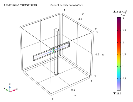
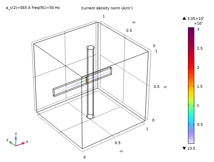
In the Settings window for Multislice, click Replace Expression in the upper-right corner of the Expression section. From the menu, choose Component 1 (comp1) > Magnetic Fields > Currents and charge > mf.normJ - Current density norm - A/m².
Streamline Multislice 1
1
In the Model Builder window, click Streamline Multislice 1.
2
In the Settings window for Streamline Multislice, click Replace Expression in the upper-right corner of the Expression section. From the menu, choose Component 1 (comp1) > Magnetic Fields > Currents and charge > mf.Jx,...,mf.Jz - Current density (spatial frame).
3
In the AC Electric Current Density toolbar, click  Plot.
The AC eddy currents circulate within the beam.
Finish by plotting the RMS displacement of the tip of the beam as a function of frequency (Figure 3).
RMS Displacement vs. Frequency
1
In the Results toolbar, click  1D Plot Group.
2
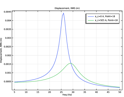
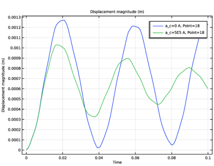
In the Settings window for 1D Plot Group, type RMS Displacement vs. Frequency in the Label text field.
3
Locate the Data section. From the Dataset list, choose Frequency-Domain Vibration Analysis/Parametric Solutions 1 (sol3).
Point Graph 1
1
Right-click RMS Displacement vs. Frequency and choose Point Graph.
2
3
In the Settings window for Point Graph, click Replace Expression in the upper-right corner of the y-Axis Data section. From the menu, choose Component 1 (comp1) > Solid Mechanics > Displacement > solid.disp_rms - Displacement, RMS - m.
4
Click to expand the Legends section. Select the Show legends checkbox.
5
In the RMS Displacement vs. Frequency toolbar, click  Plot.
Compare the resulting plot with that shown in Figure 3.
Now add a transient study to the model for comparison.
Add Study
1
In the Home toolbar, click  Add Study to open the Add Study window.
2
Go to the Add Study window.
3
Find the Studies subsection. In the Select Study tree, select General Studies > Stationary.
4
Click the Add Study button in the window toolbar.
5
In the Home toolbar, click  Add Study to close the Add Study window.
Time-Dependent Analysis
In the Settings window for Study, type Time-Dependent Analysis in the Label text field.
Parametric Sweep
1
In the Study toolbar, click  Parametric Sweep.
2
In the Settings window for Parametric Sweep, locate the Study Settings section.
3
4
Step 1: Stationary
1
In the Model Builder window, click Step 1: Stationary.
2
In the Settings window for Stationary, locate the Physics and Variables Selection section.
3
In the Solve for column of the table, under Component 1 (comp1), clear the checkbox for Solid Mechanics (solid).
4
In the Solve for column of the table, under Component 1 (comp1) > Multiphysics, clear the checkbox for Magnetomechanics, Solid 1 (mmcpl1).
Step 2: Time Dependent
1
In the Study toolbar, click  Time Dependent.
2
In the Settings window for Time Dependent, locate the Study Settings section.
3
In the Output times text field, type range(0,0.001,0.1).
4
Locate the Physics and Variables Selection section. Select the Modify model configuration for study step checkbox.
5
In the tree, select Component 1 (comp1) > Solid Mechanics (solid) > Harmonic Boundary Load for Frequency-Domain Vibration Analysis.
6
To significantly reduce the computation time, it is also possible to tweak tolerances and solve the magnetic fields problem with a direct solver, since the air domain has a finite conductivity and the induced current acts as a gauge.
7
Locate the Study Settings section. From the Tolerance list, choose User controlled.
Solution 6 (sol6)
1
In the Study toolbar, click  Show Default Solver.
2
In the Model Builder window, expand the Solution 6 (sol6) node.
3
In the Model Builder window, expand the Time-Dependent Analysis > Solver Configurations > Solution 6 (sol6) > Dependent Variables 2 node, then click Magnetic Vector Potential (Spatial Frame) (comp1.A).
4
In the Settings window for Field, locate the Scaling section.
5
From the Method list, choose None.
6
In the Model Builder window, under Time-Dependent Analysis > Solver Configurations > Solution 6 (sol6) > Dependent Variables 2 click Filtering Variable (comp1.mf.coil1.Vf).
7
In the Settings window for Field, locate the Scaling section.
8
From the Method list, choose None.
9
In the Study toolbar, click  Compute.
Results
Magnetic Flux Density (mf)
1
In the Magnetic Flux Density (mf) toolbar, click  Plot.
The first default plot from the second study again shows the static magnetic field around a current carrying wire; compare with Figure 2.
The next plot shows the von Mises stress in the beam at the end of the transient study.
Stress (solid) 1
1
In the Model Builder window, click Stress (solid) 1.
2
In the Stress (solid) 1 toolbar, click  Plot.
Finish by the displacement of the tip of the beam as a function of time (Figure 5).
Displacement vs. Time
1
In the Results toolbar, click  1D Plot Group.
2
In the Settings window for 1D Plot Group, type Displacement vs. Time in the Label text field.
3
Locate the Data section. From the Dataset list, choose Time-Dependent Analysis/Parametric Solutions 2 (sol8).
Point Graph 1
1
Right-click Displacement vs. Time and choose Point Graph.
2
3
In the Settings window for Point Graph, locate the y-Axis Data section.
4
In the Expression text field, type solid.disp.
5
Locate the Legends section. Select the Show legends checkbox.
6
In the Displacement vs. Time toolbar, click  Plot.