PDF

Induction Heating Including Curie Temperature and Movement
Introduction
Induction heating is used for various metallurgical processes such as hardening. Here, the 3D induction heating of a mechanical joint passing through an induction heating coil is simulated. Curie point effects and temperature-dependent resistivity in the iron are taken into account.
Figure 1: External current density (red streamlines) and prescribed velocity of the mechanical joint (blue arrow).The joint is surrounded by air, separated into one moving part (inner) and one stationary part (outer).
Model Definition
The problem is set up in a 3D modeling space and the geometry sequence is imported from a reference file. The model consists of a mechanical joint moving through a current-conducting coil as viewed in Figure 1 using the Prescribed Deformation interface. The magnetic field is solved for in the entire model using the Magnetic Fields interface and the temperature in the joint is found using Heat Transfer in Solids. The temperature and magnetic field are coupled using Electromagnetic Heating. Symmetries are utilized to only model a quarter of the mechanical joint and its surroundings. Two studies are performed: the first solves for the magnetic field in the frequency domain, while the second solves the full transient model over one minute, using the first solution as the initial magnetic field.
The model takes the temperature-dependent resistivity into consideration. Curie point effects are also included, the temperature above which the magnetic properties of a material are lost.
A Note On The Use Of Magnetic Continuity In 3D
The geometry in this model uses an assembly, rather than a union. This is to accommodate for the moving domains (the mechanical joint) and the stationary domains (the coil). The assembly consists of two parts with disjoint meshes. A Moving Mesh is used to apply the motion. Since the two parts are not naturally connected, a continuity constraint will need to be added for the magnetic fields. To achieve this, the Magnetic Fields interface uses the Magnetic Continuity feature.
The Magnetic Fields interface uses curl elements to solve for the magnetic vector potential in 3D. As a consequence, enforcing the continuity directly between the two sliding meshes (Adst = Asrc pointwise) will not guarantee current conservation. Unless when handled correctly (using conforming meshes and specific time steps) Ampère’s Law may be violated. To allow for a nonconforming sliding mesh, an auxiliary scalar potential is introduced on the connecting boundary. It enforces the conditions:
(1)
where the second equation is imposed via a suitable stabilization algorithm that shares the same topological properties as using the Magnetic Fields, No Currents magnetic scalar potential.
Results and Discussion
The frequency-domain solution for the magnetic flux density norm and generated heat in the mechanical joint is shown in Figure 2. The heat is concentrated to the part of the joint directly underneath the external current. Skin effects are visible for the magnetic flux density.
For the transient study, the temperature evolution of a selection of points is shown in Figure 3, the corresponding points are displayed in Figure 4. The temperature and magnetic flux density after 30 seconds is shown in Figure 5. Here, the displacement of the mechanical joint is also clear. A cross section of the temperature distribution at the final time point is shown in Figure 6 together with the maximum reached temperature at each point of the same cross section.
Figure 2: The stationary electromagnetic heat and magnetic flux density norm on the 2D slice.
Figure 3: Temperature evolution of some selected points on the moving joint. The selected points are shown in Figure 4
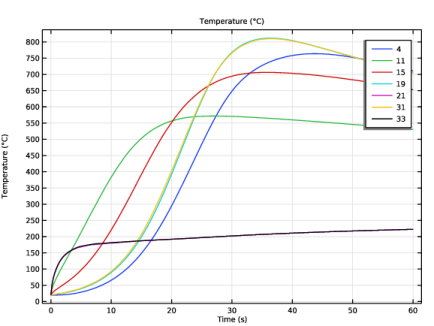
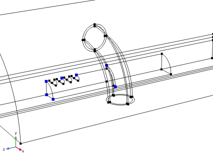
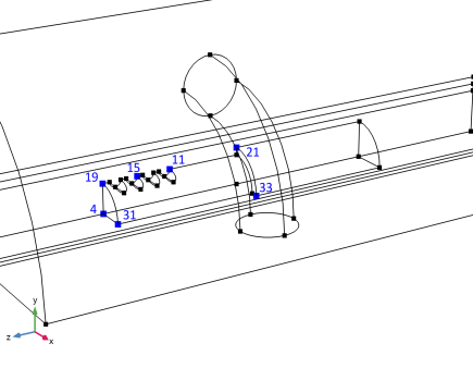
. The edge points 4, 19, and 31 reach the highest temperatures.
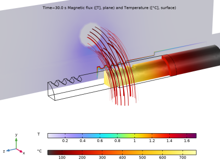
Figure 4: The selected points for the temperature evolution in Figure 3.
Figure 5: Temperature distribution of the joint, external current density (arrows), and magnetic flux density norm (slice) at t = 30 s.
Figure 6: Cross section of the maximum reached temperature at each point in the joint and the temperature at t = 60 s in the transient study.
Application Library path: ACDC_Module/Electromagnetic_Heating/induction_heating_curie_movement
Modeling Instructions
From the File menu, choose New.
New
In the New window, click  Model Wizard.
Model Wizard
1
In the Model Wizard window, click  3D.
2
In the Select Physics tree, select AC/DC > Electromagnetic Fields > Magnetic Fields (mf).
3
Click Add.
4
In the Select Physics tree, select Heat Transfer > Heat Transfer in Solids (ht).
5
Click Add.
6
In the Select Physics tree, select Mathematics > Deformed Mesh > Moving Mesh > Prescribed Deformation.
7
Click Add.
8
Click  Study.
9
In the Select Study tree, select Preset Studies for Some Physics Interfaces > Frequency Domain.
10
Global Definitions
Parameters 1
1
In the Model Builder window, under Global Definitions click Parameters 1.
2
In the Settings window for Parameters, locate the Parameters section.
3
Click  Load from File.
4
Interpolation 1 (int1)
1
In the Home toolbar, click  Functions and choose Global > Interpolation.
2
In the Settings window for Interpolation, locate the Definition section.
3
In the Function name text field, type murOfB.
4
Click  Load from File.
5
6
Locate the Units section. In the Function table, enter the following settings:
7
In the Argument table, enter the following settings:
Step 1 (step1)
1
In the Home toolbar, click  Functions and choose Global > Step.
2
In the Settings window for Step, type CuriePermFact in the Function name text field.
3
Locate the Parameters section. In the Location text field, type 273.15+(Tc-273.15)/2.
4
In the From text field, type 1.
5
In the To text field, type 0.
6
Click to expand the Smoothing section. In the Size of transition zone text field, type (Tc-273.15).
7
From the Number of continuous derivatives list, choose 1.
Step 2 (CuriePermFact2)
1
Right-click Step 1 (CuriePermFact) and choose Duplicate.
2
In the Settings window for Step, type Conductivity in the Function name text field.
3
Locate the Parameters section. In the From text field, type 6e6.
4
In the To text field, type 1e6.
Gaussian Pulse 1 (gp1)
1
In the Home toolbar, click  Functions and choose Global > Gaussian Pulse.
2
In the Settings window for Gaussian Pulse, type CurieHeatFact in the Function name text field.
3
Locate the Parameters section. In the Location text field, type Tc.
4
In the Standard deviation text field, type 100.
5
In the Integral value text field, type 1[K].
Geometry 1
With the global definitions in order, construct the geometry. The geometry will utilize symmetries and consist of only a quarter of the full joint with its surroundings.
Work Plane 1 (wp1)
1
In the Model Builder window, expand the Component 1 (comp1) > Geometry 1 node.
2
Right-click Geometry 1 and choose Work Plane.
3
In the Settings window for Work Plane, locate the Plane Definition section.
4
From the Plane list, choose zx-plane.
Work Plane 1 (wp1) > Plane Geometry
In the Model Builder window, click Plane Geometry.
Work Plane 1 (wp1) > Rectangle 1 (r1)
1
In the Work Plane toolbar, click  Rectangle.
2
In the Settings window for Rectangle, locate the Size and Shape section.
3
In the Width text field, type 0.4.
4
In the Height text field, type 0.09.
5
Locate the Position section. In the xw text field, type -0.2.
6
In the yw text field, type 0.035.
7
Click to expand the Layers section. In the table, enter the following settings:
Work Plane 1 (wp1) > Circle 1 (c1)
1
In the Work Plane toolbar, click  Circle.
2
In the Settings window for Circle, locate the Size and Shape section.
3
In the Radius text field, type 0.02.
4
Locate the Position section. In the xw text field, type 0.02.
5
In the yw text field, type 0.07.
6
Click to expand the Layers section. In the table, enter the following settings:
Revolve 1 (rev1)
1
In the Model Builder window, right-click Geometry 1 and choose Revolve.
2
In the Settings window for Revolve, locate the Revolution Angles section.
3
Click the Angles button.
4
In the End angle text field, type 90.
5
Locate the Revolution Axis section. Find the Direction of revolution axis subsection. In the xw text field, type 1.
6
In the yw text field, type 0.
All stationary domains have now been constructed. Now, to the moving domains.
Work Plane 2 (wp2)
1
In the Geometry toolbar, click  Work Plane.
2
In the Settings window for Work Plane, locate the Plane Definition section.
3
From the Plane list, choose zx-plane.
4
Locate the Unite Objects section. Clear the Unite objects checkbox.
Work Plane 2 (wp2) > Plane Geometry
In the Model Builder window, click Plane Geometry.
Work Plane 2 (wp2) > Rectangle 1 (r1)
1
In the Work Plane toolbar, click  Rectangle.
2
In the Settings window for Rectangle, locate the Size and Shape section.
3
In the Width text field, type 0.7.
4
In the Height text field, type 0.035.
5
Locate the Position section. In the xw text field, type -0.2.
6
Locate the Layers section. In the table, enter the following settings:
7
Clear the Layers on bottom checkbox.
8
Select the Layers on top checkbox.
Work Plane 2 (wp2) > Rectangle 2 (r2)
1
In the Work Plane toolbar, click  Rectangle.
2
In the Settings window for Rectangle, locate the Size and Shape section.
3
In the Width text field, type 0.1.
4
In the Height text field, type 0.025.
5
Locate the Position section. In the xw text field, type -0.1.
Work Plane 2 (wp2) > Rectangle 3 (r3)
1
In the Work Plane toolbar, click  Rectangle.
2
In the Settings window for Rectangle, locate the Size and Shape section.
3
In the Width text field, type 0.1.
4
In the Height text field, type 0.02.
Work Plane 2 (wp2) > Union 1 (uni1)
1
In the Work Plane toolbar, click  Booleans and Partitions and choose Union.
2
Select the objects r2 and r3 only.
3
In the Settings window for Union, locate the Union section.
4
Clear the Keep interior boundaries checkbox.
Revolve 2 (rev2)
1
In the Model Builder window, right-click Geometry 1 and choose Revolve.
2
In the Settings window for Revolve, locate the Revolution Angles section.
3
Click the Angles button.
4
In the End angle text field, type 90.
5
Locate the Revolution Axis section. Find the Direction of revolution axis subsection. In the xw text field, type 1.
6
In the yw text field, type 0.
Next, some ridges in the mechanical joint will be constructed.
Cylinder 1 (cyl1)
1
In the Geometry toolbar, click  Cylinder.
2
In the Settings window for Cylinder, locate the Size and Shape section.
3
In the Radius text field, type 0.004.
4
In the Height text field, type 0.05.
5
Locate the Position section. In the y text field, type 0.02.
6
In the z text field, type 0.055.
7
Locate the Axis section. From the Axis type list, choose x-axis.
Array 1 (arr1)
1
In the Geometry toolbar, click  Transforms and choose Array.
2
3
In the Settings window for Array, locate the Size section.
4
In the z size text field, type 4.
5
Locate the Displacement section. In the z text field, type 0.012.
Ferromagnetic Domain
1
In the Geometry toolbar, click  Booleans and Partitions and choose Difference.
2
In the Settings window for Difference, type Ferromagnetic Domain in the Label text field.
3
Click the  Zoom Extents button in the Graphics toolbar.
4
Click the  Wireframe Rendering button in the Graphics toolbar.
5
Select the object rev2(2) only.
6
Locate the Difference section. Click to select the  Activate Selection toggle button for Objects to subtract.
7
Select the objects arr1(1,1,1), arr1(1,1,2), arr1(1,1,3), and arr1(1,1,4) only. That is, all four small cylinders.
8
Locate the Selections of Resulting Entities section. Select the Resulting objects selection checkbox.
9
Click  Build Selected.
Moving Domains
1
In the Geometry toolbar, click  Booleans and Partitions and choose Union.
2
In the Settings window for Union, type Moving Domains in the Label text field.
3
Select the objects dif1 and rev2(1) only.
4
Locate the Selections of Resulting Entities section. Select the Resulting objects selection checkbox.
Now, the geometry is just about finished. What remains is forming an assembly, which is done by changing the (default) Form Union node.
Form Union (fin)
1
In the Model Builder window, under Component 1 (comp1) > Geometry 1 click Form Union (fin).
2
In the Settings window for Form Union/Assembly, locate the Form Union/Assembly section.
3
From the Action list, choose Form an assembly.
4
Clear the Fast pair detection for stacked objects checkbox.
5
In the Geometry toolbar, click  Build All.
6
Click the  Show Grid button in the Graphics toolbar.
7
Click the  Go to Default View button in the Graphics toolbar.
Compare the wireframe rendering of the geometry with the figure above. Note that mirror symmetries will be utilized, which is why only a quarter of the full mechanical part is modeled. Note also that an Identity Boundary Pair node was automatically added under Definitions. This is a result of forming an assembly instead of a union while finalizing the geometry and is generally necessary when working with moving parts. Next, create some selections.
Definitions
Adjacent 1
1
In the Definitions toolbar, click  Adjacent.
2
In the Settings window for Adjacent, locate the Input Entities section.
3
Under Input selections, click  Add.
4
In the Add dialog, select Ferromagnetic Domain in the Input selections list.
5
Explicit 1
1
In the Definitions toolbar, click  Explicit.
2
In the Settings window for Explicit, locate the Input Entities section.
3
From the Geometric entity level list, choose Boundary.
4
Difference 1
1
In the Definitions toolbar, click  Difference.
2
In the Settings window for Difference, locate the Geometric Entity Level section.
3
From the Level list, choose Boundary.
4
Locate the Input Entities section. Under Selections to add, click  Add.
5
In the Add dialog, select Adjacent 1 in the Selections to add list.
6
7
In the Settings window for Difference, locate the Input Entities section.
8
Under Selections to subtract, click  Add.
9
In the Add dialog, select Explicit 1 in the Selections to subtract list.
10
Coil
1
In the Definitions toolbar, click  Explicit.
2
In the Settings window for Explicit, type Coil in the Label text field.
3
Input
1
In the Definitions toolbar, click  Cylinder.
2
In the Settings window for Cylinder, type Input in the Label text field.
3
Locate the Geometric Entity Level section. From the Level list, choose Boundary.
4
Locate the Size and Shape section. In the Outer radius text field, type 0.02.
5
In the Top distance text field, type 0.
6
In the Bottom distance text field, type 0.
7
Locate the Position section. In the x text field, type 0.07.
8
In the z text field, type 0.02.
9
Locate the Axis section. From the Axis type list, choose y-axis.
10
Locate the Output Entities section. From the Include entity if list, choose All vertices inside cylinder.
Output
1
Right-click Input and choose Duplicate.
2
In the Settings window for Cylinder, type Output in the Label text field.
3
Locate the Position section. In the x text field, type 0.
4
In the y text field, type 0.07.
5
Locate the Axis section. From the Axis type list, choose x-axis.
Create two new views.
View 4
1
In the Model Builder window, right-click Definitions and choose View.
2
In the Settings window for View, locate the View section.
3
Select the Wireframe rendering checkbox.
4
Clear the Show grid checkbox.
5
Select the Lock camera checkbox.
Camera
1
In the Model Builder window, expand the View 4 node, then click Camera.
2
In the Settings window for Camera, locate the Camera section.
3
In the Zoom angle text field, type 9.
4
Locate the Position section. In the x text field, type 1.4.
5
In the y text field, type 0.4.
6
In the z text field, type 3.7.
7
Locate the Up Vector section. In the x text field, type 0.
8
In the y text field, type 1.
9
In the z text field, type 0.
10
Locate the View Offset section. In the x text field, type 0.
11
In the y text field, type 0.
12
Click  Update.
View 5
In the Model Builder window, under Component 1 (comp1) > Definitions right-click View 4 and choose Duplicate.
Camera
1
In the Model Builder window, expand the View 5 node, then click Camera.
2
In the Settings window for Camera, locate the Camera section.
3
In the Zoom angle text field, type 16.
4
Locate the Position section. In the x text field, type 0.9.
5
In the z text field, type 0.55.
6
Locate the Target section. In the x text field, type 0.
7
In the y text field, type 0.
8
In the z text field, type 0.
9
Locate the Center of Rotation section. In the x text field, type 0.
10
In the y text field, type 0.
11
In the z text field, type 0.
12
Click  Update.
13
In the Graphics window toolbar, clicknext to  Go to Default View, then choose Go to View 4.
The identity boundary pair was automatically configured with the correct boundary selections when the assembly was formed in the geometry. Look at these selections by clicking on the Identity Boundary Pair node.
Identity Boundary Pair 1 (ap1)
In the Model Builder window, under Component 1 (comp1) > Definitions click Identity Boundary Pair 1 (ap1).
Moving Mesh
Prescribed Deformation 1
1
In the Model Builder window, under Component 1 (comp1) > Moving Mesh click Prescribed Deformation 1.
2
In the Settings window for Prescribed Deformation, locate the Geometric Entity Selection section.
3
From the Selection list, choose Moving Domains.
4
Locate the Prescribed Deformation section. Specify the dx vector as
Next, configure the magnetic fields interface. Start by changing from the default quadratic discretization to linear.
Magnetic Fields (mf)
1
In the Model Builder window, under Component 1 (comp1) click Magnetic Fields (mf).
2
In the Settings window for Magnetic Fields, click to expand the Discretization section.
3
From the Magnetic vector potential list, choose Linear.
Free Space 1
1
In the Model Builder window, under Component 1 (comp1) > Magnetic Fields (mf) click Free Space 1.
2
In the Settings window for Free Space, locate the Stabilization section.
3
From the σstab list, choose User defined.
Magnetic Continuity 1
1
In the Physics toolbar, click  Pairs and choose Magnetic Continuity.
2
In the Settings window for Magnetic Continuity, locate the Pair Selection section.
3
4
In the Add dialog, select Identity Boundary Pair 1 (ap1) in the Pairs list.
5
Domain Coil 1
1
In the Physics toolbar, click  Domains and choose Domain Coil.
2
In the Settings window for Domain Coil, locate the Domain Selection section.
3
From the Selection list, choose Coil.
4
Locate the Coil section. In the Icoil text field, type I0.
5
In the Model Builder window, expand the Domain Coil 1 node.
Input 1
1
In the Model Builder window, expand the Component 1 (comp1) > Magnetic Fields (mf) > Domain Coil 1 > Geometry Analysis 1 node, then click Input 1.
2
In the Settings window for Input, locate the Boundary Selection section.
3
From the Selection list, choose Input.
Geometry Analysis 1
In the Model Builder window, click Geometry Analysis 1.
Output 1
1
In the Physics toolbar, click  Attributes and choose Output.
2
In the Settings window for Output, locate the Boundary Selection section.
3
From the Selection list, choose Output.
For the final addition to the Magnetic Fields interface, create the domain for the mechanical joint where the Curie point effects will be introduced.
Ampère’s Law in Solids 1
1
In the Physics toolbar, click  Domains and choose Ampère’s Law in Solids.
2
In the Settings window for Ampère’s Law in Solids, locate the Domain Selection section.
3
From the Selection list, choose Ferromagnetic Domain.
4
Locate the Constitutive Relation B-H section. From the μr list, choose User defined. In the associated text field, type 1+murOfB(mf.normB)*CuriePermFact(T).
Heat Transfer in Solids (ht)
1
In the Model Builder window, under Component 1 (comp1) click Heat Transfer in Solids (ht).
2
In the Settings window for Heat Transfer in Solids, locate the Domain Selection section.
3
From the Selection list, choose Ferromagnetic Domain.
4
Click to expand the Discretization section. From the Temperature list, choose Linear.
Solid 1
1
In the Model Builder window, under Component 1 (comp1) > Heat Transfer in Solids (ht) click Solid 1.
2
In the Settings window for Solid, locate the Thermodynamics, Solid section.
3
From the Cp list, choose User defined. In the associated text field, type (440+2e5*CurieHeatFact(T))*1[J/(kg*K)].
Continuity 1
1
In the Model Builder window, click Continuity 1.
2
In the Settings window for Continuity, locate the Advanced section.
3
Select the Disconnect pair checkbox.
Heat Flux 1
1
In the Physics toolbar, click  Boundaries and choose Heat Flux.
2
In the Settings window for Heat Flux, locate the Boundary Selection section.
3
From the Selection list, choose Difference 1.
4
Locate the Heat Flux section. From the Flux type list, choose Convective heat flux.
5
In the h text field, type 10.
Surface-to-Ambient Radiation 1
1
In the Physics toolbar, click  Boundaries and choose Surface-to-Ambient Radiation.
2
In the Settings window for Surface-to-Ambient Radiation, locate the Boundary Selection section.
3
From the Selection list, choose Difference 1.
4
Locate the Surface-to-Ambient Radiation section. From the ε list, choose User defined. In the associated text field, type 0.9.
Multiphysics
Electromagnetic Heating 1 (emh1)
1
In the Physics toolbar, click  Multiphysics Couplings and choose Domain > Electromagnetic Heating.
2
In the Settings window for Electromagnetic Heating, locate the Domain Selection section.
3
From the Selection list, choose Ferromagnetic Domain.
4
Locate the Boundary Selection section. Click  Clear Selection.
Add Material from Library
In the Home toolbar, click  Windows and choose Add Material from Library.
Add Material
1
Go to the Add Material window.
2
In the tree, select Built-in > Air.
3
Click the Add to Component button in the window toolbar.
4
In the tree, select Built-in > Iron.
5
Click the Add to Component button in the window toolbar.
6
In the tree, select Built-in > Copper.
7
Click the Add to Component button in the window toolbar.
8
In the Home toolbar, click  Add Material to close the Add Material window.
Materials
Copper (mat3)
1
In the Settings window for Material, locate the Geometric Entity Selection section.
2
From the Selection list, choose Coil.
Iron (mat2)
1
In the Model Builder window, click Iron (mat2).
2
In the Settings window for Material, locate the Geometric Entity Selection section.
3
From the Selection list, choose Ferromagnetic Domain.
Mesh 1
1
In the Model Builder window, under Component 1 (comp1) click Mesh 1.
2
In the Settings window for Mesh, locate the Sequence Type section.
3
From the list, choose User-controlled mesh.
4
In the Mesh toolbar, click  Clear Sequence.
Mapped 1
1
In the Mesh toolbar, click  More Generators and choose Mapped.
2
In the Settings window for Mapped, locate the Boundary Selection section.
3
From the Selection list, choose Input.
4
Click the  Go to Default View button in the Graphics toolbar.
5
Click the  Zoom to Selection button in the Graphics toolbar.
Distribution 1
1
Right-click Mapped 1 and choose Distribution.
2
3
In the Settings window for Distribution, locate the Distribution section.
4
In the Number of elements text field, type 2.
Distribution 2
1
In the Model Builder window, right-click Mapped 1 and choose Distribution.
2
3
In the Settings window for Distribution, locate the Distribution section.
4
In the Number of elements text field, type 3.
Swept 1
1
In the Mesh toolbar, click  Swept.
2
In the Settings window for Swept, locate the Domain Selection section.
3
From the Geometric entity level list, choose Domain.
4
Distribution 1
1
Right-click Swept 1 and choose Distribution.
2
Right-click Distribution 1 and choose Build Selected.
3
In the Settings window for Distribution, in the Graphics window toolbar, clicknext to  Go to Default View, then choose Go to View 5.
Free Tetrahedral 1
In the Mesh toolbar, click  Free Tetrahedral.
Size 1
1
Right-click Free Tetrahedral 1 and choose Size.
2
In the Settings window for Size, locate the Geometric Entity Selection section.
3
From the Geometric entity level list, choose Domain.
4
From the Selection list, choose Ferromagnetic Domain.
5
Locate the Element Size section. Click the Custom button.
6
Locate the Element Size Parameters section.
7
Select the Maximum element size checkbox. In the associated text field, type del_sat*2.
Size 2
1
Right-click Size 1 and choose Duplicate.
2
In the Settings window for Size, locate the Geometric Entity Selection section.
3
From the Geometric entity level list, choose Boundary.
4
From the Selection list, choose Difference 1.
5
Locate the Element Size Parameters section. In the Maximum element size text field, type del_sat.
6
Select the Maximum element growth rate checkbox. In the associated text field, type 1.1.
Size 3
1
In the Model Builder window, right-click Free Tetrahedral 1 and choose Size.
2
In the Settings window for Size, in the Graphics window toolbar, clicknext to  Go to Default View, then choose Go to View 4.
3
Locate the Geometric Entity Selection section. From the Geometric entity level list, choose Domain.
4
5
Locate the Element Size section. Click the Custom button.
6
Locate the Element Size Parameters section.
7
Select the Maximum element size checkbox. In the associated text field, type 0.01.
8
Select the Minimum element size checkbox. In the associated text field, type 0.01.
Boundary Layers 1
1
In the Mesh toolbar, click  Boundary Layers.
2
In the Settings window for Boundary Layers, locate the Geometric Entity Selection section.
3
From the Geometric entity level list, choose Domain.
4
From the Selection list, choose Ferromagnetic Domain.
Boundary Layer Properties
1
In the Model Builder window, click Boundary Layer Properties.
2
In the Settings window for Boundary Layer Properties, locate the Boundary Selection section.
3
From the Selection list, choose Difference 1.
4
Locate the Layers section. In the Number of layers text field, type 3.
5
From the Thickness specification list, choose First layer.
6
In the Thickness text field, type del_sat/10.
7
In the Model Builder window, right-click Mesh 1 and choose Build All.
8
In the Settings window for Mesh, in the Graphics window toolbar, clicknext to  Go to Default View, then choose Go to View 4.
Initialization (Magnetic)
1
In the Model Builder window, click Study 1.
2
In the Settings window for Study, type Initialization (Magnetic) in the Label text field.
3
Locate the Study Settings section. Clear the Generate default plots checkbox.
Step 2: Coil Geometry Analysis
1
In the Study toolbar, click  More Study Steps and choose Other > Coil Geometry Analysis.
2
Drag and drop above Step 2: Frequency Domain.
Step 2: Frequency Domain
1
In the Model Builder window, click Step 2: Frequency Domain.
2
In the Settings window for Frequency Domain, locate the Study Settings section.
3
In the Frequencies text field, type f.
Solution 1 (sol1)
1
In the Study toolbar, click  Show Default Solver.
2
In the Model Builder window, expand the Solution 1 (sol1) node, then click Compile Equations: Frequency Domain.
3
In the Settings window for Compile Equations, locate the Study and Step section.
4
Select the Split complex variables in real and imaginary parts checkbox.
5
Results
Initialization
1
In the Model Builder window, expand the Results node.
2
Right-click Results and choose 3D Plot Group.
3
In the Settings window for 3D Plot Group, type Initialization in the Label text field.
4
Locate the Plot Settings section. From the View list, choose View 5.
5
Locate the Color Legend section. Select the Show units checkbox.
Volume 1
1
Right-click Initialization and choose Volume.
2
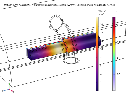
In the Settings window for Volume, click Replace Expression in the upper-right corner of the Expression section. From the menu, choose Component 1 (comp1) > Magnetic Fields > Heating and losses > mf.Qrh - Volumetric loss density, electric - W/m³.
3
Locate the Expression section. In the Unit field, type W/cm^3.
4
Locate the Coloring and Style section. From the Color table list, choose HeatCamera.
Selection 1
1
Right-click Volume 1 and choose Selection.
2
In the Settings window for Selection, locate the Selection section.
3
From the Selection list, choose Ferromagnetic Domain.
Slice 1
1
In the Model Builder window, right-click Initialization and choose Slice.
2
In the Settings window for Slice, locate the Plane Data section.
3
From the Entry method list, choose Coordinates.
4
Locate the Coloring and Style section. From the Color table list, choose Prism.
Deformation 1
1
Right-click Slice 1 and choose Deformation.
2
In the Settings window for Deformation, locate the Expression section.
3
In the x-component text field, type -1.
Selection 1
1
In the Model Builder window, right-click Slice 1 and choose Selection.
2
In the Settings window for Selection, locate the Selection section.
3
From the Selection list, choose Ferromagnetic Domain.
4
In the Initialization toolbar, click  Plot and compare the resulting plot with Figure 2.
Add Study
1
In the Home toolbar, click  Add Study to open the Add Study window.
2
Go to the Add Study window.
3
Find the Studies subsection. In the Select Study tree, select Preset Studies for Selected Multiphysics > Frequency–Transient.
4
Click the Add Study button in the window toolbar.
5
In the Home toolbar, click  Add Study to close the Add Study window.
Induction Heating Moving Load
1
In the Settings window for Study, type Induction Heating Moving Load in the Label text field.
2
Locate the Study Settings section. Clear the Generate default plots checkbox.
Step 2: Coil Geometry Analysis
1
In the Study toolbar, click  More Study Steps and choose Other > Coil Geometry Analysis.
2
Drag and drop above Step 2: Frequency–Transient.
The Coil Geometry Analysis study step only calculates a scalar potential for the current in the coil. The remaining dependent variables (for example the magnetic vector potential and the temperature) will be taken from the initialization study.
3
In the Settings window for Coil Geometry Analysis, click to expand the Values of Dependent Variables section.
4
Find the Values of variables not solved for subsection. From the Settings list, choose User controlled.
5
From the Method list, choose Solution.
6
From the Study list, choose Initialization (Magnetic), Frequency Domain.
Step 2: Frequency–Transient
1
In the Model Builder window, click Step 2: Frequency–Transient.
2
In the Settings window for Frequency–Transient, locate the Study Settings section.
3
In the Output times text field, type range(0,0.2,5) range(5.5,0.5,60).
4
In the Frequency text field, type f.
This frequency-transient study combines a time-dependent study for the Heat Transfer in Solids interface with a frequency study for the Magnetic Fields interface. The time-averaged heating from the magnetic fields will be used to calculate the temperature in the transient study. At each time step, the temperature will be used to calculate a new magnetic field which, consequently, gives a new value for the heat. Before computing, however, the default solver should be modified slightly to properly handle the nonlinearities in the model.
Solution 3 (sol3)
1
In the Study toolbar, click  Show Default Solver.
2
In the Model Builder window, expand the Solution 3 (sol3) node, then click Compile Equations: Frequency–Transient.
3
In the Settings window for Compile Equations, locate the Study and Step section.
4
Select the Split complex variables in real and imaginary parts checkbox.
5
In the Model Builder window, under Induction Heating Moving Load > Solver Configurations > Solution 3 (sol3) click Dependent Variables 2.
6
In the Settings window for Dependent Variables, locate the Scaling section.
7
From the Method list, choose Initial-value based.
8
In the Model Builder window, under Induction Heating Moving Load > Solver Configurations > Solution 3 (sol3) click Time-Dependent Solver 1.
9
In the Settings window for Time-Dependent Solver, click to expand the Time Stepping section.
10
From the Steps taken by solver list, choose Strict.
11
Right-click Induction Heating Moving Load > Solver Configurations > Solution 3 (sol3) > Time-Dependent Solver 1 and choose Fully Coupled.
12
In the Settings window for Fully Coupled, click to expand the Method and Termination section.
13
From the Jacobian update list, choose On every iteration.
14
Results
Point Temperatures
1
In the Results toolbar, click  1D Plot Group.
2
In the Settings window for 1D Plot Group, type Point Temperatures in the Label text field.
3
Locate the Data section. From the Dataset list, choose Induction Heating Moving Load/Solution 3 (sol3).
Point Graph 1
1
Right-click Point Temperatures and choose Point Graph.
2
In the Settings window for Point Graph, in the Graphics window toolbar, clicknext to  Go to Default View, then choose Go to View 5.
3
4
Locate the y-Axis Data section. In the Expression text field, type T.
5
From the Unit list, choose °C.
6
Click to expand the Legends section. Select the Show legends checkbox.
7
In the Point Temperatures toolbar, click  Plot.
Compare the temperatures with Figure 3. Next, create some datasets for the remaining plot groups. The first new dataset will be using the Material (X, Y, Z) frame with a selection of the ferromagnetic domain. This reference frame ignores the translation from the moving mesh, which allows an analysis of the moving part without it moving out of frame. Furthermore, the symmetries of the model will now be utilized using the Mirror 3D dataset.
Induction Heating Moving Load/Solution 2 (Ferromagnetic Domain)
1
In the Model Builder window, expand the Results > Datasets node.
2
Right-click Results > Datasets > Induction Heating Moving Load/Solution 3 (sol3) and choose Duplicate.
3
In the Settings window for Solution, type Induction Heating Moving Load/Solution 2 (Ferromagnetic Domain) in the Label text field.
4
Locate the Solution section. From the Frame list, choose Material  (X, Y, Z).
Selection
1
In the Results toolbar, click  Attributes and choose Selection.
2
In the Settings window for Selection, locate the Geometric Entity Selection section.
3
From the Geometric entity level list, choose Domain.
4
From the Selection list, choose Ferromagnetic Domain.
Mirror 3D 1
1
In the Results toolbar, click  More Datasets and choose Mirror 3D.
2
In the Settings window for Mirror 3D, locate the Data section.
3
From the Dataset list, choose Induction Heating Moving Load/Solution 2 (Ferromagnetic Domain) (sol3).
4
Locate the Plane Data section. From the Plane list, choose ZX-planes.
Mirror 3D 2
1
In the Results toolbar, click  More Datasets and choose Mirror 3D.
2
In the Settings window for Mirror 3D, locate the Data section.
3
From the Dataset list, choose Mirror 3D 1.
Initialization (Magnetic)/Solution 1 (Current Domain)
1
In the Model Builder window, under Results > Datasets right-click Initialization (Magnetic)/Solution 1 (sol1) and choose Duplicate.
2
In the Settings window for Solution, type Initialization (Magnetic)/Solution 1 (Current Domain) in the Label text field.
Selection
1
In the Results toolbar, click  Attributes and choose Selection.
2
In the Settings window for Selection, locate the Geometric Entity Selection section.
3
From the Geometric entity level list, choose Domain.
4
From the Selection list, choose Coil.
Surface Temperature
1
In the Results toolbar, click  3D Plot Group.
2
In the Settings window for 3D Plot Group, type Surface Temperature in the Label text field.
3
Locate the Data section. From the Dataset list, choose Mirror 3D 2.
4
From the Time (s) list, choose Last (60).
5
Click to expand the Title section. From the Title type list, choose Custom.
6
Find the User subsection. In the Suffix text field, type Temperature [°C].
7
Find the Type and data subsection. Clear the Type checkbox.
8
Clear the Description checkbox.
9
Clear the Unit checkbox.
10
Find the Layout subsection. Clear the Use parameter indicator for solution and phase checkbox.
11
Locate the Plot Settings section. From the View list, choose View 5.
Surface 1
1
Right-click Surface Temperature and choose Surface.
2
In the Settings window for Surface, locate the Expression section.
3
In the Expression text field, type T.
4
From the Unit list, choose °C.
5
Locate the Coloring and Style section. From the Color table list, choose GrayBody.
6
In the Surface Temperature toolbar, click  Plot.
Surface Temperature
In the Model Builder window, click Surface Temperature.
Max/Min Surface 1
1
In the Surface Temperature toolbar, click  More Plots and choose Max/Min Surface.
2
In the Settings window for Max/Min Surface, locate the Expression section.
3
In the Expression text field, type T.
4
From the Unit list, choose °C.
5
Locate the Display section. From the Display list, choose Max.
6
Locate the Text Format section. In the Prefix text field, type Temperature, .
7
Select the Include unit checkbox.
8
In the Precision text field, type 3.
9
Locate the Coloring and Style section. From the Color list, choose Magenta.
10
In the Surface Temperature toolbar, click  Plot.
Max/Min Surface 2
1
Right-click Max/Min Surface 1 and choose Duplicate.
2
In the Settings window for Max/Min Surface, locate the Expression section.
3
In the Expression text field, type mf.Qrh.
4
From the Unit list, choose MW/m^3.
5
Locate the Text Format section. In the Prefix text field, type Heat, .
6
In the Precision text field, type 1.
7
In the Surface Temperature toolbar, click  Plot.
Compare the surface temperature and wireframe with the figure below.
Surface 1
1
In the Results toolbar, click  More Datasets and choose Surface.
2
In the Settings window for Surface, locate the Data section.
3
From the Dataset list, choose Induction Heating Moving Load/Solution 2 (Ferromagnetic Domain) (sol3).
4
Locate the Parameterization section. From the x- and y-axes list, choose ZY-plane.
5
Temperature Cross Sections
1
In the Results toolbar, click  2D Plot Group.
2
In the Settings window for 2D Plot Group, type Temperature Cross Sections in the Label text field.
3
Click to expand the Title section. From the Title type list, choose Manual.
4
From the Number format list, choose Engineering.
5
Select the Show trailing zeros checkbox.
6
In the Precision text field, type 3.
7
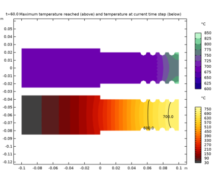
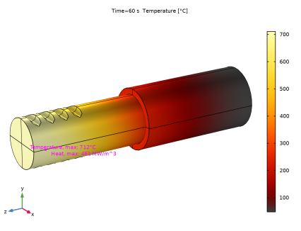
In the Title text area, type Maximum temperature reached (above) and temperature at current time step (below).
8
In the Parameter indicator text field, type t=eval(t).
9
Locate the Plot Settings section. Clear the Plot dataset edges checkbox.
10
Locate the Color Legend section. Select the Show units checkbox.
11
From the Position list, choose Right double.
Contour 1
1
Right-click Temperature Cross Sections and choose Contour.
2
In the Settings window for Contour, locate the Expression section.
3
In the Expression text field, type min(attimemax(0,t,T,max(0,T-700[degC]))+700[degC],900[degC]).
4
From the Unit list, choose °C.
5
Locate the Levels section. From the Entry method list, choose Levels.
6
In the Levels text field, type range(600,25,850).
7
Locate the Coloring and Style section. From the Contour type list, choose Filled.
8
From the Color table list, choose AuroraBorealis.
9
From the Color table transformation list, choose Reverse.
Contour 2
1
Right-click Contour 1 and choose Duplicate.
2
In the Settings window for Contour, click to expand the Title section.
3
From the Title type list, choose None.
4
Locate the Coloring and Style section. Clear the Color legend checkbox.
Deformation 1
1
Right-click Contour 2 and choose Deformation.
2
In the Settings window for Deformation, locate the Expression section.
3
In the x-component text field, type 0.
4
In the y-component text field, type -2*y.
5
Locate the Scale section.
6
Select the Scale factor checkbox. In the associated text field, type 1.
Temperature Cross Sections
Right-click Deformation 1 and choose Contour.
Contour 3
1
In the Settings window for Contour, locate the Expression section.
2
In the Expression text field, type T.
3
From the Unit list, choose °C.
4
Locate the Levels section. From the Entry method list, choose Levels.
5
In the Levels text field, type range(30,30,800).
6
Locate the Coloring and Style section. From the Contour type list, choose Filled.
7
From the Color table list, choose GrayBody.
Deformation 1
1
Right-click Contour 3 and choose Deformation.
2
In the Settings window for Deformation, locate the Expression section.
3
In the x-component text field, type 0.
4
In the y-component text field, type -2*Y-0.06.
5
Locate the Scale section.
6
Select the Scale factor checkbox. In the associated text field, type 1.
Contour 4
1
Right-click Contour 3 and choose Duplicate.
2
In the Settings window for Contour, locate the Coloring and Style section.
3
Clear the Color legend checkbox.
Deformation 1
1
In the Model Builder window, expand the Contour 4 node, then click Deformation 1.
2
In the Settings window for Deformation, locate the Expression section.
3
In the y-component text field, type -0.06.
Contour 5
1
In the Model Builder window, right-click Temperature Cross Sections and choose Contour.
2
In the Settings window for Contour, locate the Expression section.
3
In the Expression text field, type T.
4
From the Unit list, choose °C.
5
Locate the Levels section. From the Entry method list, choose Levels.
6
In the Levels text field, type 600 700.
7
Locate the Coloring and Style section. Select the Level labels checkbox.
8
From the Coloring list, choose Uniform.
9
From the Color list, choose Black.
10
Clear the Color legend checkbox.
Deformation 1
1
Right-click Contour 5 and choose Deformation.
2
In the Settings window for Deformation, locate the Expression section.
3
In the x-component text field, type 0.
4
In the y-component text field, type -2*Y-0.06.
5
Locate the Scale section.
6
Select the Scale factor checkbox. In the associated text field, type 1.
Contour 6
1
In the Model Builder window, under Results > Temperature Cross Sections right-click Contour 5 and choose Duplicate.
2
In the Settings window for Contour, click to expand the Inherit Style section.
3
From the Plot list, choose Contour 5.
4
Locate the Coloring and Style section. Clear the Level labels checkbox.
Deformation 1
1
In the Model Builder window, expand the Contour 6 node, then click Deformation 1.
2
In the Settings window for Deformation, locate the Expression section.
3
In the y-component text field, type -0.06.
4
In the Temperature Cross Sections toolbar, click  Plot.
5
Click the  Zoom Extents button in the Graphics toolbar.
Compare the plot with Figure 6 and create a new animation of the temperature evolution in the ferromagnetic domain.
Animation 1
In the Temperature Cross Sections toolbar, click  Animation and choose Player.
Time Dependent
1
In the Results toolbar, click  3D Plot Group.
2
In the Settings window for 3D Plot Group, type Time Dependent in the Label text field.
3
Locate the Data section. From the Dataset list, choose Induction Heating Moving Load/Solution 3 (sol3).
4
From the Time (s) list, choose Interpolation.
5
In the Time text field, type 30.
6
Locate the Title section. From the Title type list, choose Custom.
7
From the Number format list, choose Engineering.
8
Select the Show trailing zeros checkbox.
9
In the Precision text field, type 3.
10
Find the User subsection. In the Suffix text field, type Magnetic flux ([T], plane) and Temperature ([°C], surface).
11
Find the Type and data subsection. Clear the Description checkbox.
12
Clear the Type checkbox.
13
Clear the Unit checkbox.
14
Find the Layout subsection. Clear the Use parameter indicator for solution and phase checkbox.
15
Locate the Plot Settings section. From the View list, choose View 5.
16
Clear the Plot dataset edges checkbox.
17
Locate the Color Legend section. Select the Show units checkbox.
18
From the Position list, choose Bottom.
Slice 1
1
Right-click Time Dependent and choose Slice.
2
In the Settings window for Slice, locate the Plane Data section.
3
From the Entry method list, choose Coordinates.
4
Locate the Coloring and Style section. From the Color table list, choose Prism.
Deformation 1
1
Right-click Slice 1 and choose Deformation.
2
In the Settings window for Deformation, locate the Expression section.
3
In the x-component text field, type -1.
4
Locate the Scale section.
5
Select the Scale factor checkbox. In the associated text field, type 0.02.
Volume 1
1
In the Model Builder window, right-click Time Dependent and choose Volume.
2
In the Settings window for Volume, locate the Expression section.
3
In the Expression text field, type T.
4
From the Unit list, choose °C.
5
Locate the Coloring and Style section. From the Color table list, choose GrayBody.
Selection 1
1
Right-click Volume 1 and choose Selection.
2
In the Settings window for Selection, locate the Selection section.
3
From the Selection list, choose Ferromagnetic Domain.
Line 1
1
In the Model Builder window, right-click Time Dependent and choose Line.
2
In the Settings window for Line, locate the Data section.
3
From the Dataset list, choose Initialization (Magnetic)/Solution 1 (sol1).
4
Locate the Expression section. In the Expression text field, type 1.
5
Locate the Coloring and Style section. From the Coloring list, choose Uniform.
6
From the Color list, choose Black.
Selection 1
1
Right-click Line 1 and choose Selection.
2
In the Settings window for Selection, locate the Selection section.
3
From the Geometric entity level list, choose Domain.
4
From the Selection list, choose Ferromagnetic Domain.
Streamline 1
1
In the Model Builder window, right-click Time Dependent and choose Streamline.
2
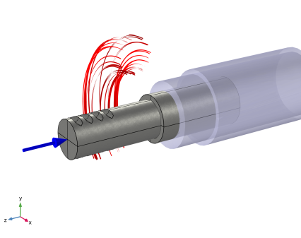
In the Settings window for Streamline, click Replace Expression in the upper-right corner of the Expression section. From the menu, choose Component 1 (comp1) > Magnetic Fields > Currents and charge > mf.Jx,...,mf.Jz - Current density (spatial frame).
3
Locate the Streamline Positioning section. From the Positioning list, choose Starting-point controlled.
4
In the Points text field, type 45.
5
Locate the Coloring and Style section. Find the Line style subsection. From the Type list, choose Ribbon.
Selection 1
1
Right-click Streamline 1 and choose Selection.
2
In the Settings window for Selection, locate the Selection section.
3
From the Selection list, choose Coil.
4
In the Time Dependent toolbar, click  Plot, and compare the plot with Figure 5. Create a new animation.
Animation 2
In the Time Dependent toolbar, click  Animation and choose Player.