|
|
|
|
1
|
|
2
|
|
3
|
Click Add.
|
|
4
|
Click
|
|
5
|
|
6
|
Click
|
|
1
|
|
2
|
|
100 Ω·m
|
|
1
|
|
2
|
|
3
|
|
4
|
|
5
|
|
6
|
|
7
|
Click to expand the Layers section. In the table, enter the following settings:
|
|
8
|
|
9
|
Select the Right checkbox.
|
|
10
|
Select the Front checkbox.
|
|
11
|
Select the Back checkbox.
|
|
12
|
Click
|
|
1
|
|
2
|
|
3
|
|
4
|
|
5
|
|
6
|
|
7
|
Click
|
|
1
|
|
2
|
|
3
|
|
4
|
|
5
|
|
6
|
|
7
|
|
8
|
|
9
|
Click
|
|
1
|
|
2
|
|
3
|
|
4
|
|
5
|
|
1
|
|
2
|
|
3
|
Locate the Definition section. In the Expression text field, type 1[A]*rho0/(2*pi)*(1/abs(x-x1)-1/abs(x-x2)).
|
|
4
|
|
1
|
|
2
|
|
3
|
|
4
|
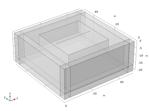
Select all the exterior boundaries located in the ground. This operation can be performed quickly by selecting the Group by continuous tangent checkbox, then clicking on one boundary from each of the sides and the bottom of the box.
|
|
5
|
|
1
|
|
3
|
|
1
|
|
3
|
|
4
|
|
5
|
Select the Interior boundaries checkbox.
|
|
6
|
|
1
|
|
2
|
|
3
|
|
4
|
|
1
|
In the Model Builder window, under Component 1 (comp1) right-click Materials and choose Blank Material.
|
|
2
|
|
4
|
|
1
|
|
3
|
|
4
|
|
5
|
|
6
|
|
7
|
Click OK.
|
|
1
|
|
2
|
|
3
|
|
1
|
|
2
|
|
3
|
|
5
|
|
6
|
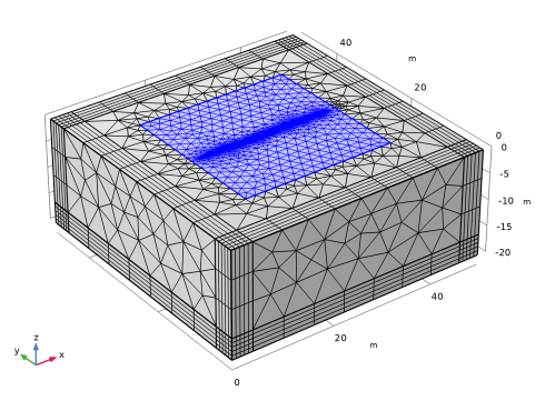
Locate the Element Size Parameters section.
|
|
7
|
|
1
|
|
3
|
|
4
|
Click the Custom button.
|
|
5
|
Locate the Element Size Parameters section.
|
|
6
|
|
7
|
Click
|
|
1
|
|
2
|
|
3
|
Select the Auxiliary sweep checkbox.
|
|
4
|
Click
|
|
6
|
Click
|
|
8
|
|
9
|
|
1
|
|
2
|
|
1
|
|
2
|
|
3
|
|
4
|
|
5
|
|
6
|
|
1
|
|
2
|
|
3
|
|
1
|
|
2
|
|
3
|
|
4
|
|
1
|
|
2
|
|
3
|
In the Expression text field, type with(1,ec.Jx)*with(2,ec.Jx)+with(1,ec.Jy)*with(2,ec.Jy)+with(1,ec.Jz)*with(2,ec.Jz).
|
|
4
|
|
5
|
|
6
|
|
7
|
|
8
|
|
9
|
|
10
|
|
11
|
|
1
|
|
2
|
|
3
|
|
4
|
|
5
|
|
1
|
|
2
|
|
1
|
|
2
|
|
3
|
|
1
|
|
2
|
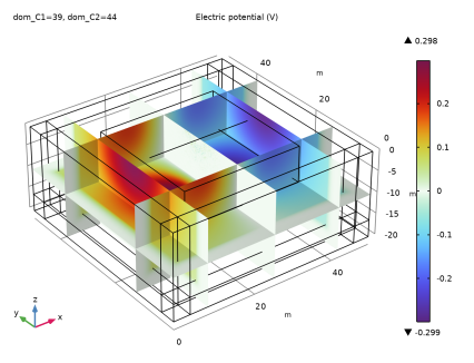
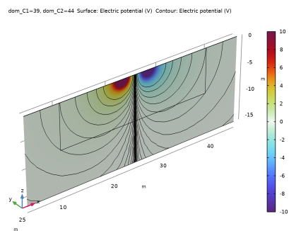
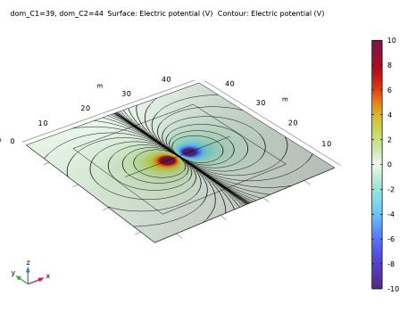
In the Settings window for 3D Plot Group, type Electric Potential at the Surface in the Label text field.
|
|
3
|
|
1
|
|
2
|
|
3
|
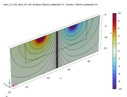
Select the Manual color range checkbox.
|
|
4
|
|
5
|
|
6
|
|
1
|
|
2
|
|
3
|
|
4
|
|
5
|
|
6
|
|
7
|
Clear the Color legend checkbox.
|
|
8
|
|
9
|
|
1
|
|
2
|
|
3
|
|
4
|
|
1
|
|
2
|
|
3
|
|
4
|
|
1
|
|
2
|
|
3
|
Select the Manual color range checkbox.
|
|
4
|
|
5
|
|
6
|
|
1
|
|
2
|
|
3
|
|
4
|
|
5
|
|
6
|
|
7
|
Clear the Color legend checkbox.
|
|
8
|
|
1
|
|
2
|
|
3
|
|
4
|
|
1
|
|
2
|
|
3
|
|
4
|
|
5
|
|
6
|
|
1
|
|
2
|
|
3
|
|
4
|
|
5
|
Locate the Plot Settings section.
|
|
6
|
|
7
|
|
1
|
|
2
|
|
3
|
|
4
|
|
5
|
|
6
|
|
7
|
|
8
|
|
9
|
|
10
|
Click to expand the Legends section.
|
|
1
|
|
2
|
|
3
|
|
4
|
|
1
|
|
2
|
|
3
|
|
4
|
|
5
|
|
6
|
|
7
|
|
1
|
|
2
|
|
3
|
|
4
|
|
5
|
|
6
|
|
7
|
|
1
|
|
2
|
|
3
|
|
4
|
|
5
|
Locate the Plot Settings section.
|
|
6
|
|
7
|
|
8
|
|
9
|
Select the y-axis log scale checkbox.
|
|
10
|
|
11
|
|
12
|
|
1
|
|
2
|
|
3
|
|
4
|
|
5
|
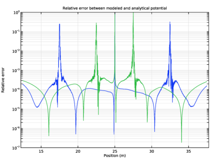
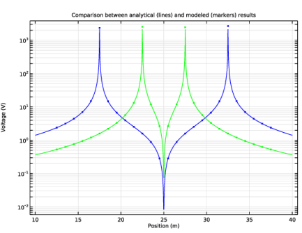
Locate the y-Axis Data section. In the Expression text field, type abs(V-V_ref(x,17.5,32.5))/abs(V).
|
|
7
|
|
8
|
|
1
|
|
2
|
|
3
|
|
4
|
Locate the y-Axis Data section. In the Expression text field, type abs(V-V_ref(x,22.5,27.5))/abs(V).
|
|
5
|