Introduction
The Acoustics Module consists of a set of physics interfaces that enable you to simulate the propagation of sound in fluids and solids in a fully multiphysics-enabled environment. The available physics interfaces include pressure acoustics, elastic waves, acoustic–solid interaction, aeroacoustics (detailed convected acoustic models and flow induced noise), thermoviscous acoustics, ultrasound, geometrical acoustics, and pipe acoustics. For acoustic analysis, covering the frequency range from infrasound to ultrasonics as well as many formulations of the underlying equations, the Acoustics Module incorporates four numerical methods, including finite elements (FEM), boundary elements (BEM), discontinuous Galerkin (dG-FEM), and ray tracing.
Figure 1: COMSOL model of the sound pressure level distribution in a muffler system.
Acoustic simulations using this module can easily solve classical problems such as scattering, diffraction, emission, radiation, and transmission of sound. These problems are relevant to muffler design, loudspeaker construction, sound insulation for absorbers and diffusers, the evaluation of directional acoustic patterns like directivity, noise radiation problems, and much more. The acoustic–structure multiphysics couplings enable modeling vibroacoustic problems involving structure- and fluid-borne sound and their interaction. For example, acoustic–structure interaction is simulated for detailed muffler design, ultrasound piezo-actuators, sonar technology, and noise and vibration analysis of machinery in the automotive industry. Using the capabilities of COMSOL Multiphysics, it is also possible to analyze and design electroacoustic transducers such as loudspeakers, sensors, microphones, and hearing aid receivers. The propagation of elastic waves can be modeled in solids and porous materials as well as in coupled problems.
Aeroacoustic problems can be analyzed and modeled by solving the linearized potential flow equations, the linearized Euler equations, or the linearized Navier–Stokes equations. These equations are used to model the one-way interaction between an external flow and an acoustic field, so-called convected acoustics. Applications range from jet-engine noise analysis to simulating acoustic flow sensors, liner systems with bias and/or grazing flow, and mufflers with flow. Flow-induced noise can be modeled using the Lighthill acoustic analogy or the aeroacoustic wave equation. This analysis requires a detailed LES or DES flow analysis available with the CFD Module. Flow data available in the CGNS format can be imported and mapped.
The Thermoviscous Acoustics interfaces can accurately model systems having small geometrical dimensions where thermal and viscous boundary layer losses are important. This is relevant to the mobile phone and hearing aid industries, for all transducer designers, and for modeling the true properties of metamaterials. For MEMS transducers, a slip-wall formulation can be added. In the time domain, nonlinear effects can also be included.
Figure 2: COMSOL model of an ultrasound flowmeter modeled using the Convected Wave Equation interface. The model includes interaction with a steady state background flow.
The Ultrasound branch includes two interfaces. The Convected Wave Equation, Time Explicit interface can be used to compute the transient propagation of linear ultrasound acoustic waves over large distances (relative to the wavelengths). The Nonlinear Pressure Acoustics, Time Explicit interface can be used to model the propagation of high amplitude nonlinear acoustic waves. Both interfaces can be coupled to the Elastic Waves, Time Explicit interface and the Piezoelectric Waves, Time Explicit multiphysics interface. The interfaces under the ultrasound branch are not restricted to high-frequency propagation but can, in general, be applied to any acoustically large problem.
Geometrical Acoustics includes the Ray Acoustics and the Acoustic Diffusion Equation interfaces. These physics interfaces are valid in the high-frequency limit where the acoustic wavelength is much smaller than the characteristic geometric features. Both interfaces are suited for modeling acoustics in rooms and concert halls. The Ray Acoustics interface can also be used, for example, in outdoor scenarios.
Dedicated functionality also exists for modeling the steady fluid flow, called Acoustic Streaming, induced by an acoustic field. Acoustic streaming is a nonlinear phenomenon that occurs due to the nonlinearity of the Navier–Stokes equations. Applications are in the biomedical industry such as lab-on-a-chip for cell sorting and more.
The Acoustics Module is of great benefit to engineers. By using 3D simulations, existing products can be optimized and new products more quickly designed with virtual prototypes. Simulations also help designers, researchers, and engineers to gain insight into problems that are difficult to handle experimentally. Also, by optimizing a design virtually before real-life testing and manufacturing it, companies save time and money.
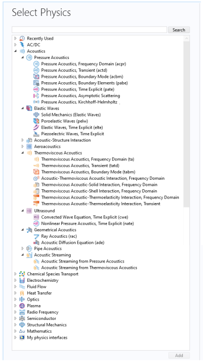
Some of the physics interfaces available with this module are shown in Figure 3 and are located under the Acoustics branch in the Model Wizard when selecting physics. The next section The Acoustics Module Physics Interfaces provides an overview of the physics interface functionality under each branch.
There are many application areas where these physics interfaces are used — from modeling simple pressure waves in air to examining complex interactions between elastic waves and pressure waves in porous materials. For a brief introduction to the basic concepts and theory of acoustics, see the Basics of Acoustics.
The Acoustics Module Application Library has many examples of applications modeling, for example sound-insulation lining, loudspeakers, microphones, and mufflers. These examples show, among other things, how to simulate acoustic losses. The loss models range from homogenized empirical fluid models for fibrous materials to those that include thermal and viscous losses in detail using the Thermoviscous Acoustics interface.
Predefined couplings can be used to model the interaction between acoustic, structural, and electric fields in piezoelectric materials (see The Application Libraries Window for information about accessing these files). You can also get started with your own COMSOL modeling by going to the tutorial Example: Absorptive Muffler.
Figure 3: The Acoustics Module physics interfaces and branches in the Select Physics wizard. Some physics interfaces require additional modules.