|
|
|


|
1
|
|
2
|
In the Select Physics tree, select Optics > Wave Optics > Electromagnetic Waves, Frequency Domain (ewfd).
|
|
3
|
Click Add.
|
|
4
|
Click
|
|
5
|
In the Select Study tree, select Preset Studies for Selected Physics Interfaces > Wavelength Domain.
|
|
6
|
Click
|
|
1
|
|
2
|
|
3
|
|
1
|
|
2
|
|
3
|
|
4
|
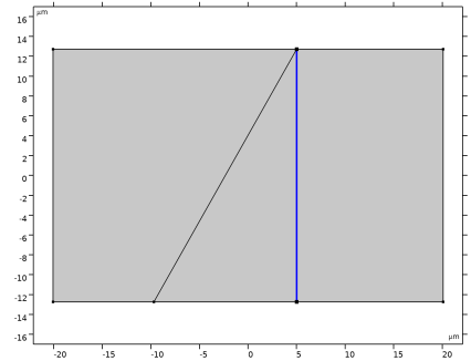
Browse to the model’s Application Libraries folder and double-click the file gaussian_beam_propagation_optical_prism_parameters_geom.txt.
|
|
1
|
|
2
|
In the Settings window for Parameters, type Anti-Reflection Coatings Parameters in the Label text field.
|
|
3
|
|
4
|
Browse to the model’s Application Libraries folder and double-click the file gaussian_beam_propagation_optical_prism_parameters_ar.txt.
|
|
1
|
|
2
|
|
3
|
|
4
|
|
5
|
|
6
|
|
1
|
|
2
|
|
3
|
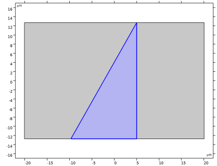
Locate the Coordinates section. In the table, enter the following settings:
|
|
4
|
|
1
|
|
2
|
Go to the Add Material window.
|
|
3
|
|
4
|
Right-click and choose Add to Component 1 (comp1).
|
|
5
|
|
1
|
In the Model Builder window, under Component 1 (comp1) right-click Materials and choose Blank Material.
|
|
2
|
|
4
|
Locate the Material Contents section. In the table, enter the following settings:
|
|
5
|
|
1
|
In the Model Builder window, under Component 1 (comp1) click Electromagnetic Waves, Frequency Domain (ewfd).
|
|
2
|
|
3
|
From the Electric field components solved for list, choose Out-of-plane vector, as the beam possesses out-of-plane electric field component only.
|
|
1
|
|
3
|
|
4
|
Click
|
|
5
|
|
6
|
Click OK.
|
|
7
|
In the Settings window for Matched Boundary Condition, locate the Matched Boundary Condition section.
|
|
8
|
|
9
|
|
10
|
|
11
|
|
12
|
|
1
|
|
2
|
|
3
|
|
4
|
|
1
|
|
3
|
|
4
|
Click
|
|
5
|
|
6
|
Click OK.
|
|
7
|
In the Settings window for Matched Boundary Condition, locate the Matched Boundary Condition section.
|
|
8
|
|
1
|
|
3
|
|
4
|
Click
|
|
5
|
|
6
|
Click OK.
|
|
7
|
In the Settings window for Matched Boundary Condition, locate the Matched Boundary Condition section.
|
|
8
|
|
1
|
|
3
|
In the Settings window for Matched Boundary Condition, locate the Matched Boundary Condition section.
|
|
4
|
|
1
|
|
3
|
In the Settings window for Transition Boundary Condition, locate the Transition Boundary Condition section.
|
|
4
|
|
5
|
|
6
|
|
1
|
|
3
|
In the Settings window for Transition Boundary Condition, locate the Transition Boundary Condition section.
|
|
4
|
|
5
|
|
6
|
|
7
|
In the Model Builder window, right-click Electromagnetic Waves, Frequency Domain (ewfd) and choose Copy, to simulate for the p-polarized Gaussian beam.
|
|
1
|
In the Model Builder window, right-click Component 1 (comp1) and choose Paste Electromagnetic Waves, Frequency Domain.
|
|
2
|
|
3
|
|
4
|
From the Electric field components solved for list, choose In-plane vector, as the beam possesses in-plane electric field components only.
|
|
1
|
In the Model Builder window, expand the Electromagnetic Waves, Frequency Domain 2 (ewfd2) node, then click Matched Boundary Condition 1.
|
|
2
|
In the Settings window for Matched Boundary Condition, locate the Matched Boundary Condition section.
|
|
3
|
|
1
|
|
2
|
In the Settings window for Transition Boundary Condition, locate the Transition Boundary Condition section.
|
|
3
|
|
4
|
|
1
|
|
2
|
In the Settings window for Transition Boundary Condition, locate the Transition Boundary Condition section.
|
|
3
|
|
4
|
|
1
|
|
2
|
|
3
|
|
4
|
|
1
|
|
2
|
|
3
|
|
1
|
|
2
|
|
3
|
|
1
|
|
2
|
In the Settings window for Variables, type Reflectance and Transmittance Calculation in the Label text field.
|
|
3
|
|
4
|
Browse to the model’s Application Libraries folder and double-click the file gaussian_beam_propagation_optical_prism_variables.txt.
|
|
1
|
|
2
|
In the Settings window for Wavelength Domain, type Wavelength Domain (s-polarization) in the Label text field.
|
|
3
|
Locate the Physics and Variables Selection section. In the Solve for column of the table, under Component 1 (comp1), clear the checkbox for Electromagnetic Waves, Frequency Domain 2 (ewfd2).
|
|
4
|
|
1
|
|
2
|
In the Settings window for Wavelength Domain, type Wavelength Domain (p-polarization) in the Label text field.
|
|
3
|
Locate the Physics and Variables Selection section. In the Solve for column of the table, under Component 1 (comp1), clear the checkbox for Electromagnetic Waves, Frequency Domain (ewfd).
|
|
4
|
In the Solve for column of the table, under Component 1 (comp1), select the checkbox for Electromagnetic Waves, Frequency Domain 2 (ewfd2).
|
|
5
|
|
1
|
|
2
|
|
1
|
|
2
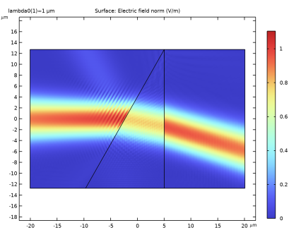
|
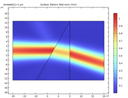
In the Settings window for 2D Plot Group, type Electric Field Norm, s-polarized Beam in the Label text field.
 |
|
1
|
|
2
|
In the Settings window for 2D Plot Group, type Electric Field Norm, p-polarized Beam in the Label text field.
 |
|
1
|
|
2
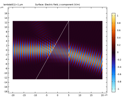
|
In the Settings window for 2D Plot Group, type Electric Field Component, s-polarized Beam in the Label text field.
|
|
1
|
In the Model Builder window, expand the Electric Field Component, s-polarized Beam node, then click Surface 1.
|
|
2
|
|
3
|
|
4
|
|
1
|
|
2
|
|
3
|
|
4
|
|
1
|
|
2
|
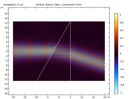
In the Settings window for 2D Plot Group, type Electric Field Component, p-polarized Beam in the Label text field.
|
|
1
|
In the Model Builder window, expand the Electric Field Component, p-polarized Beam node, then click Surface 1.
|
|
2
|
|
3
|
 ,
, ,
, ,
, ,
,