PDF

Michelson Interferometer
Introduction
A Michelson interferometer is composed of five elements: two mirrors, one beam splitter, an imaging device (screen), and a coherent light source. Figure 1 shows and describes a basic Michelson interferometer arrangement, the interference pattern is generated when the rays reflected by mirrors M1 and M2 arrive at the screen with different optical path lengths.
Changing, even slightly, the optical path length of either beam results in a change of the interference pattern at the screen. This change of optical path length can be accomplished by moving one of the mirrors. Unexpected changes in optical path length can also occur if any of the device’s optical components undergo deformation, such as thermal expansion. This model illustrates the effects of thermal expansion on the interference pattern obtained at the screen of the interferometer.
Figure 1: An illuminated Michelson interferometer arrangement with the resulting interference pattern displayed on the screen (S). The light comes from the light source(LS), hits the beam splitter (BS) before being equally diverted toward mirror 1 (M1) and mirror 2 (M2). Once reflected at the mirrors, the two composing beams return to the beam splitter (BS) where they recombine to travel toward the screen (S) or the light source (LS).
 
 
Model Definition
In this model the rays propagate through the beam splitter and the air enclosing the optical components. The mirrors are treated as Wall boundary conditions at which specular reflection occurs. The beam splitter (BS) is composed of two BK7 glass prisms separated by a thin dielectric film (BS interface). The beam splitter is surrounded by an anti-reflective (AR) coating. The AR coating and the BS interface are modeled by applying the Thin Dielectric Film subnode to the Material Discontinuity node.
The Settings window for the Material Discontinuity node includes an option to automatically set up a single-layer coating with the desired reflectance. In this case, a reflectance of 0.5 is desired for the interior boundary of the beam splitter so that an incoming ray is divided into two rays of equal intensity.
The light source used in the model is a He-Ne laser. For sake of simplicity only one ray is initially released from a point on a face of the enclosure. The initial ray is polarized such that it forms an s-polarized wave at the beam splitter surface. For the interference pattern to be accurate, it must correspond to a wavefront that subtends a very small solid angle. This can be accomplished by setting initial radius of curvature of the wavefront to 1 m and setting the initial optical path length difference between the beam splitter and the two mirrors to a large multiple of the free-space wavelength.
The interference pattern obtained at the screen depends on the radii of curvature, phase, and angle of incidence of the two rays as they arrive at the screen. For a spherical wavefront with principal radius of curvature r1,0 with normal incidence at a surface, the change in phase corresponding to a shift xp in position on the screen is
where k is the wave number. Similarly, the change in phase for a wavefront with principal radius of curvature r2,0 is
For small values of xp, an approximate solution for the difference in phase between the two wavefronts can be obtained by taking a Taylor series expansion of the expressions for ΔΨ1 and ΔΨ2 and retaining terms of up to second order in xp,
If the two rays interfere constructively at xp = 0, they also interfere constructively where the phase difference between the two wavefronts is an integer multiple of 2π. The first such point occurs where
(1)
which is the distance from the center of the interference pattern to a point of maximum intensity on the first fringe.
Figure 2: Interference of coherent light emitted from two point sources separated by a small distance.
Results and Discussion
Figure 3 shows the interference pattern resulting from the combination of two rays having an optical path length difference of δd = 8000 λ0. As expected for spherical waves, the interference fringes are circular. On the figure it is possible to approximate the distance from the center of the screen to the radial position of greatest intensity on the first circular fringe.
Figure 3: Interference pattern obtained for an optical path length difference of δd = 8000 λ0.
Reference
1. M. Born and E. Wolf, Principle of Optics, 7th ed., Cambridge University Press, 2011.
Application Library path: Ray_Optics_Module/Spectrometers_and_Monochromators/michelson_interferometer
Modeling Instructions
From the File menu, choose New.
New
In the New window, click  Model Wizard.
Model Wizard
1
In the Model Wizard window, click  3D.
2
In the Select Physics tree, select Optics > Ray Optics > Geometrical Optics (gop).
3
Click Add.
4
Click  Study.
5
In the Select Study tree, select Preset Studies for Selected Physics Interfaces > Ray Tracing.
6
Global Definitions
Parameters 1
1
In the Model Builder window, under Global Definitions click Parameters 1.
2
In the Settings window for Parameters, locate the Parameters section.
3
Part Libraries
1
In the Home toolbar, click  Part Libraries.
2
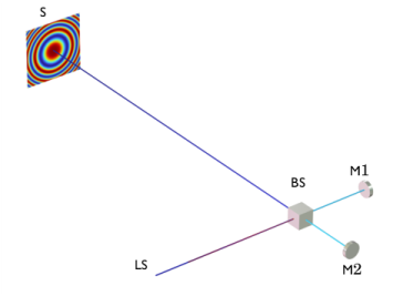
In the Part Libraries window, select Ray Optics Module > 3D > Beam Splitters > beam_splitter_cube in the tree.
3
Click  Add to Geometry.
Geometry 1
Beam Splitter Cube 1 (pi1)
1
In the Model Builder window, under Component 1 (comp1) > Geometry 1 click Beam Splitter Cube 1 (pi1).
2
In the Settings window for Part Instance, locate the Input Parameters section.
3
Cylinder 1 (cyl1)
1
In the Geometry toolbar, click  Cylinder.
2
In the Settings window for Cylinder, locate the Size and Shape section.
3
In the Radius text field, type dia/2.
4
In the Height text field, type th.
5
Locate the Position section. In the y text field, type -d2-th.
6
Locate the Axis section. From the Axis type list, choose y-axis.
Cylinder 2 (cyl2)
1
In the Geometry toolbar, click  Cylinder.
2
In the Settings window for Cylinder, locate the Size and Shape section.
3
In the Radius text field, type dia/2.
4
In the Height text field, type th.
5
Locate the Position section. In the x text field, type d1.
6
Locate the Axis section. From the Axis type list, choose x-axis.
7
Click  Build Selected.
8
Click the  Zoom Extents button in the Graphics toolbar.
Block 1 (blk1)
1
In the Geometry toolbar, click  Block.
2
In the Settings window for Block, locate the Size and Shape section.
3
In the Width text field, type 4*dia.
4
In the Depth text field, type th.
5
In the Height text field, type 4*dia.
6
Locate the Position section. From the Base list, choose Center.
7
In the y text field, type dE+th/2.
Block 2 (blk2)
1
In the Geometry toolbar, click  Block.
2
In the Settings window for Block, locate the Size and Shape section.
3
In the Width text field, type 200[mm].
4
In the Depth text field, type 450[mm].
5
In the Height text field, type 100[mm].
6
Locate the Position section. From the Base list, choose Center.
7
In the y text field, type 100[mm].
Form Union (fin)
1
In the Geometry toolbar, click  Build All.
2
Click the  Go to Default View button in the Graphics toolbar.
Definitions
View 1
In the Model Builder window, expand the Component 1 (comp1) > Definitions node, then click View 1.
Hide for Geometry 1
1
In the View 1 toolbar, click  Hide.
2
In the Settings window for Hide for Geometry, locate the Selection section.
3
From the Geometric entity level list, choose Boundary.
4
Click the  Transparency button in the Graphics toolbar.
5
On the object fin, select Boundaries 1–5 and 33 only.
Add Material
1
In the Home toolbar, click  Add Material to open the Add Material window.
2
Go to the Add Material window.
3
In the tree, select Built-in > Air.
4
Click the Add to Component button in the window toolbar.
5
In the tree, select Optical > Schott Glass > Schott N-BK7 Glass.
6
Click the Add to Component button in the window toolbar.
7
In the Home toolbar, click  Add Material to close the Add Material window.
Materials
Schott N-BK7 Glass (mat2)
Select Domains 4 and 5 only.
Geometrical Optics (gop)
1
In the Model Builder window, under Component 1 (comp1) click Geometrical Optics (gop).
2
In the Settings window for Geometrical Optics, locate the Intensity Computation section.
3
From the Intensity computation list, choose Compute intensity and power.
4
Select the Compute phase checkbox.
Material Discontinuity 1
Apply an anti-reflective coating to the outside of the beam splitter.
1
In the Model Builder window, under Component 1 (comp1) > Geometrical Optics (gop) click Material Discontinuity 1.
2
In the Settings window for Material Discontinuity, locate the Coatings section.
3
From the Thin dielectric films on boundary list, choose Anti-reflective coating.
4
Select the Treat as single layer dielectric film checkbox.
5
In the λ0 text field, type lam.
Ray Properties 1
1
In the Model Builder window, click Ray Properties 1.
2
In the Settings window for Ray Properties, locate the Ray Properties section.
3
In the λ0 text field, type lam.
Wall 1
1
In the Physics toolbar, click  Boundaries and choose Wall.
2
Mirror 1
1
In the Physics toolbar, click  Boundaries and choose Mirror.
2
Beam Splitter
Use a second Material Discontinuity node for the interior boundary of the beam splitter.
1
In the Physics toolbar, click  Boundaries and choose Material Discontinuity.
2
In the Settings window for Material Discontinuity, type Beam Splitter in the Label text field.
3
Locate the Coatings section. From the Thin dielectric films on boundary list, choose Specify reflectance.
4
In the R text field, type 0.5.
5
Select the Treat as single layer dielectric film checkbox.
6
In the n text field, type n_int.
7
In the λ0 text field, type lam.
8
In the θi text field, type 45[deg].
9
Release from Grid 1
Specify how the ray is going to be released. Release a single ray from the face of the enclosure facing mirror M1. Generate a fully polarized, -1 m radius of curvature spherical wave.
1
In the Physics toolbar, click  Global and choose Release from Grid.
2
In the Settings window for Release from Grid, locate the Initial Coordinates section.
3
In the qx,0 text field, type -100[mm].
4
Locate the Ray Direction Vector section. Specify the L0 vector as
5
Locate the Initial Radii of Curvature section. From the Wavefront shape list, choose Spherical wave.
6
In the r0 text field, type -1[m].
7
Locate the Initial Polarization section. From the Initial polarization type list, choose Fully polarized.
8
From the Initial polarization list, choose User defined.
9
Specify the u vector as
Ray Termination 1
1
In the Physics toolbar, click  Global and choose Ray Termination.
2
In the Settings window for Ray Termination, locate the Termination Criteria section.
3
From the Spatial extents of ray propagation list, choose Bounding box, from geometry.
Mesh 1
1
In the Model Builder window, under Component 1 (comp1) click Mesh 1.
2
In the Settings window for Mesh, locate the Physics-Controlled Mesh section.
3
From the Element size list, choose Coarser.
4
Click  Build All.
Study 1
Step 1: Ray Tracing
1
In the Model Builder window, under Study 1 click Step 1: Ray Tracing.
2
In the Settings window for Ray Tracing, locate the Study Settings section.
3
Click  Range.
4
In the Range dialog, type 0.1 in the Step text field.
5
In the Stop text field, type 2.2.
6
Click Replace.
7
In the Study toolbar, click  Compute.
Results
Create a dataset to display the interference pattern on the screen.
Cut Plane 1
1
In the Results toolbar, click  Cut Plane.
2
In the Settings window for Cut Plane, locate the Data section.
3
From the Dataset list, choose Ray 1.
4
Locate the Plane Data section. From the Plane list, choose xz-planes.
5
In the y-coordinate text field, type dE.
Interference Pattern
1
In the Results toolbar, click  2D Plot Group.
2
In the Settings window for 2D Plot Group, type Interference Pattern in the Label text field.
3
Locate the Data section. From the Dataset list, choose Cut Plane 1.
Interference Pattern 1
1
In the Interference Pattern toolbar, click  More Plots and choose Interference Pattern.
2
In the Settings window for Interference Pattern, locate the Coordinate Range section.
3
From the Origin location specification list, choose At ray of greatest intensity.
4
In the Interference Pattern toolbar, click  Plot. The plot should look like Figure 3.