








PDF

Transmission Line Parameters of a Coaxial Cable
Introduction
Transmission lines are used to guide waves of alternating current and voltage at radio frequencies and have been used for more than 150 years, starting with the first telegraph cables in the 1850s. Today, transmission lines exist in a variety of forms, many of which are adapted for easy fabrication and employment in printed circuit board designs. Transmission lines are key elements in most modern electronic devices. They are used to carry information, at minimal loss and distortion, from one place to another within a device and between devices. The theoretical foundation for designing and analyzing transmission lines was laid by James Clerk Maxwell, Lord Kelvin, and Oliver Heaviside. Transmission line theory is a cornerstone in the teaching of RF and microwave engineering.
Electromagnetic fields propagate along transmission lines, to a fair approximation, as transverse electromagnetic (TEM) waves. The 1D, frequency domain wave equation for the electric potential on a transmission line is written in the form:
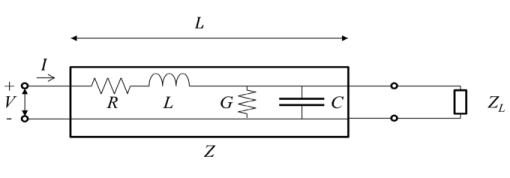
where R, L, G, and C are the distributed resistance, inductance, conductance, and capacitance, respectively. A similar wave equation can be deduced for the current flowing along the transmission line. Below is an equivalent circuit model of a transmission line terminated by a load impedance.
Figure 1: Schematic of a transmission line with a load impedance.
The solution to the wave equation represents a forward- and a backward-propagating wave:
where γ, the complex propagation constant is given by:
If only a forward-propagating wave is present in the transmission line (no reflections), dividing the voltage V by the current I gives the characteristic impedance Z, or wave impedance of the transmission line:
The design of a transmission line is to a large extent about achieving a value of the characteristic impedance that matches the impedance of the load or whatever device the transmission line is connected to. By matching the impedance, reflections are kept to a minimum and the transferred RF power is maximized.
The Transmission Line, RLGC Parameters, a predefined multiphysics interface, offers a couple of physics interfaces and multiphysics coupling for computing the transmission line parameters R, L, G, and C, as well as γ and Z for a cross section of various types of transmission lines.
Model Definition
The analysis performed by the Transmission Line, RLGC parameters interface is based on the assumption of quasi-TEM modes, meaning that longitudinal components of electric and magnetic fields are nonzero but small. Then, the main properties of the propagating mode can be deduced from separate magnetic and electric analyses, the former yielding the R and L parameters and the latter yielding the G and C parameters. The equations solved for are firstly a magnetic formulation for out-of-plane currents where the out-of-plane magnetic vector potential Az is calculated from the Magnetic Fields interface in 2D. The equation solved is:
where σ is the conductivity, ε0εr the permittivity, μ the permeability, and ω is the angular frequency. Furthermore, V0/L represents the applied out-of-plane electric field, which is applied only to the conductors. An important parameter is the skin depth:
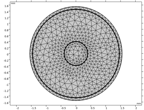
The skin depth is a measure of the exponential drop in current density with the distance to the surface inside conductors. It can be very small and needs to be resolved by the finite element mesh. This is obtained by using a special meshing method known as boundary layer meshing automatically provided by the physics-controlled mesh. After solving, the net current I flowing in the out-of-plane direction is measured by integration of the current density J:
over the forward conductor. The resulting out-of-plane impedance Z is computed as:
yielding the R and L parameters.
Secondly, a current balance for the in-plane conduction and displacement currents with the electric potential V as the unknown is solved:
A potential difference V1 is applied between the forward and return conductors and the net in-plane current I1 flowing between the conductors is measured by integration of the normal component of the in-plane current density J1:
over the surface (boundary) of the electrode with the applied potential. The resulting in-plane admittance Y1 is then computed as:
yielding the G and C parameters.
Results and Discussion
After completing the computation, the transmission line parameters in Table 1 are automatically evaluated by default, including series resistance R, series inductance L, shunt conductance G, shunt capacitance C, all calculated per unit length, as well as characteristic impedance Z and propagation constant γ.
4.2 Ω/m
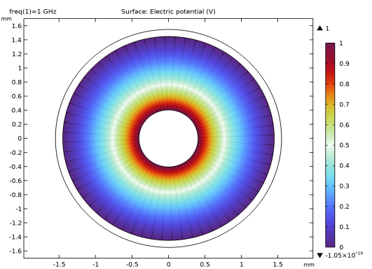
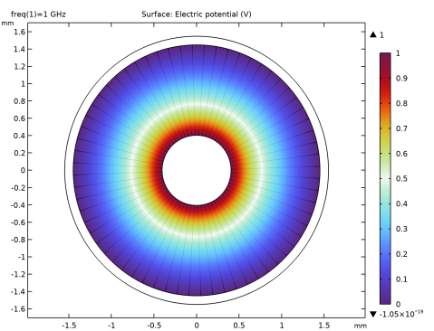
Several default plots help to understand the electromagnetic field behavior within the transmission line structure.
Figure 2: Surface plot of the electric potential along with a streamline plot of the electric field.
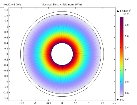
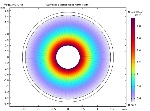
Figure 3: Surface plot of the electric field norm along with a streamline plot of the electric field.
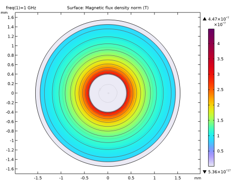
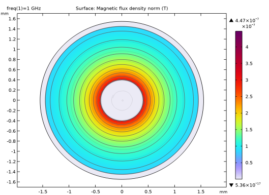
Figure 4: Surface plot of the magnetic flux density norm along with a streamline plot of the magnetic flux density and a contour plot of the z-component of the magnetic vector potential.
Notes About the COMSOL Implementation
The TEM waves assumption underlying the Transmission Line, RLGC Parameters multiphysics interface is only valid if the distance between forward (signal path) and return (ground) conductors is substantially smaller than the wavelength in the medium (<10%).
Application Library path: RF_Module/Transmission_Lines_and_Waveguides/transmission_line_coaxial
Modeling Instructions
From the File menu, choose New.
New
In the New window, click  Model Wizard.
Model Wizard
1
In the Model Wizard window, click  2D.
2
In the Select Physics tree, select Radio Frequency > Transmission Line, RLGC Parameters.
3
Click Add.
4
Click  Study.
5
In the Select Study tree, select Preset Studies for Selected Multiphysics > Frequency Domain.
6
Study 1
Step 1: Frequency Domain
1
In the Model Builder window, under Study 1 click Step 1: Frequency Domain.
2
In the Settings window for Frequency Domain, locate the Study Settings section.
3
In the Frequencies text field, type f0.
Global Definitions
Parameters 1
1
In the Model Builder window, under Global Definitions click Parameters 1.
2
In the Settings window for Parameters, locate the Parameters section.
3
Geometry 1
1
In the Model Builder window, under Component 1 (comp1) click Geometry 1.
2
In the Settings window for Geometry, locate the Units section.
3
From the Length unit list, choose mm.
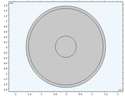
Circle 1 (c1)
1
In the Geometry toolbar, click  Circle.
2
In the Settings window for Circle, locate the Size and Shape section.
3
In the Radius text field, type Ro_coax+d_s_coax.
Circle 2 (c2)
1
In the Geometry toolbar, click  Circle.
2
In the Settings window for Circle, locate the Size and Shape section.
3
In the Radius text field, type Ro_coax.
Circle 3 (c3)
1
In the Geometry toolbar, click  Circle.
2
In the Settings window for Circle, locate the Size and Shape section.
3
In the Radius text field, type Ri_coax.
4
Click  Build All Objects.
Materials
Conductor Material
1
In the Model Builder window, under Component 1 (comp1) right-click Materials and choose Blank Material.
2
In the Settings window for Material, type Conductor Material in the Label text field.
3
Locate the Material Contents section. In the table, enter the following settings:
Dielectric Material
1
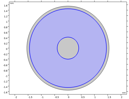
Right-click Materials and choose Blank Material.
2
In the Settings window for Material, type Dielectric Material in the Label text field.
3
4
Locate the Material Contents section. In the table, enter the following settings:
Electric Currents (ec)
1
In the Model Builder window, under Component 1 (comp1) click Electric Currents (ec).
2
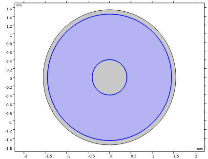
Electric Potential 1
1
In the Model Builder window, under Component 1 (comp1) > Electric Currents (ec) click Electric Potential 1.
2
In the Settings window for Electric Potential, locate the Boundary Selection section.
3
Click  Clear Selection.
4
Ground 1
1
In the Model Builder window, click Ground 1.
2
Magnetic Fields (mf)
External Current Density 1
1
In the Model Builder window, under Component 1 (comp1) > Magnetic Fields (mf) click External Current Density 1.
2
3
In the Settings window for External Current Density, locate the External Current Density section.
4
Specify the Je vector as
Perfect Magnetic Conductor 1
1
In the Model Builder window, click Perfect Magnetic Conductor 1.
2
3
Right-click Perfect Magnetic Conductor 1 and choose Disable.
Mesh 1
1
In the Model Builder window, under Component 1 (comp1) right-click Mesh 1 and choose Build All.
2
In the Home toolbar, click  Compute.
Results
Transmission Line Parameters (tlp1)
1
In the Model Builder window, under Results click Transmission Line Parameters (tlp1).
2
In the Transmission Line Parameters (tlp1) toolbar, click  Evaluate.
Electric Potential (ec)
In the Model Builder window, click Electric Potential (ec).
Electric Field (ec)
In the Model Builder window, click Electric Field (ec).
Magnetic Flux Density (mf)
In the Model Builder window, click Magnetic Flux Density (mf).