|
|
|
|
1
|
|
2
|
|
3
|
Click Add.
|
|
4
|
Click
|
|
5
|
|
6
|
Click
|
|
1
|
|
2
|
|
3
|
|
4
|
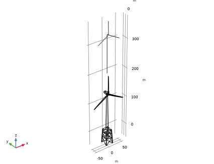
Browse to the model’s Application Libraries folder and double-click the file lightning_surge_wind_farm_turbine_tower.mphbin.
|
|
5
|
Click
|
|
6
|
Click
|
|
7
|
|
8
|
Locate the Selections of Resulting Entities section. Find the Cumulative selection subsection. Click New.
|
|
9
|
|
10
|
Click OK.
|
|
1
|
|
2
|
|
3
|
|
4
|
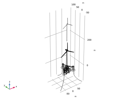
Browse to the model’s Application Libraries folder and double-click the file lightning_surge_wind_farm_turbine_blades.mphbin.
|
|
5
|
Click
|
|
6
|
|
1
|
|
2
|
|
3
|
|
4
|
Browse to the model’s Application Libraries folder and double-click the file lightning_surge_wind_farm_inner_strip.mphbin.
|
|
5
|
Click
|
|
6
|
Click
|
|
7
|
|
8
|
Locate the Selections of Resulting Entities section. Find the Cumulative selection subsection. Click New.
|
|
9
|
|
10
|
Click OK.
|
|
1
|
|
2
|
|
3
|
|
4
|
Browse to the model’s Application Libraries folder and double-click the file lightning_surge_wind_farm_turbine_support1.mphbin.
|
|
5
|
Click
|
|
6
|
|
7
|
Locate the Selections of Resulting Entities section. Find the Cumulative selection subsection. From the Contribute to list, choose Steel Body.
|
|
1
|
|
2
|
|
3
|
|
4
|
Browse to the model’s Application Libraries folder and double-click the file lightning_surge_wind_farm_turbine_support2.mphbin.
|
|
5
|
Click
|
|
6
|
|
7
|
Locate the Selections of Resulting Entities section. Find the Cumulative selection subsection. From the Contribute to list, choose Steel Body.
|
|
1
|
|
2
|
|
3
|
|
4
|
Browse to the model’s Application Libraries folder and double-click the file lightning_surge_wind_farm_water.mphbin.
|
|
5
|
Click
|
|
6
|
|
1
|
|
2
|
Select the object imp5 only.
|
|
3
|
|
4
|
|
5
|
Click
|
|
1
|
|
2
|
Select the object imp3 only.
|
|
3
|
|
4
|
|
5
|
Click
|
|
1
|
|
2
|
Select the object imp4 only.
|
|
3
|
|
4
|
|
5
|
|
6
|
Click
|
|
1
|
|
2
|
|
3
|
|
4
|
|
5
|
|
6
|
|
7
|
|
8
|
Locate the Selections of Resulting Entities section. Find the Cumulative selection subsection. From the Contribute to list, choose Steel Body.
|
|
9
|
|
1
|
|
2
|
|
3
|
|
4
|
|
5
|
|
6
|
|
7
|
|
8
|
|
9
|
Click
|
|
10
|
|
1
|
|
2
|
|
3
|
|
4
|
Browse to the model’s Application Libraries folder and double-click the file lightning_surge_wind_farm_table.txt.
|
|
5
|
|
6
|
Locate the Selections of Resulting Entities section. Find the Cumulative selection subsection. Click New.
|
|
7
|
|
8
|
Click OK.
|
|
1
|
|
2
|
|
3
|
On the object pol1, select Point 1 only.
|
|
4
|
|
5
|
On the object copy1(5), select Point 273 only.
|
|
6
|
Locate the Selections of Resulting Entities section. Find the Cumulative selection subsection. From the Contribute to list, choose Lightning Channel.
|
|
7
|
|
1
|
|
2
|
|
3
|
|
4
|
|
5
|
|
6
|
|
1
|
|
2
|
Select the object imp6 only.
|
|
3
|
|
4
|
|
5
|
Select the object cyl2 only.
|
|
6
|
Select the Keep tool objects checkbox.
|
|
7
|
Click
|
|
1
|
|
2
|
On the object par1, select Boundaries 1 and 2 only.
|
|
3
|
|
4
|
|
5
|
|
6
|
|
7
|
Clear the Automatic detection of small details checkbox.
|
|
1
|
|
2
|
Go to the Add Material window.
|
|
3
|
|
4
|
Click the Add to Component button in the window toolbar.
|
|
5
|
|
1
|
In the Model Builder window, under Component 1 (comp1) right-click Materials and choose Blank Material.
|
|
2
|
|
4
|
Locate the Material Contents section. In the table, enter the following settings:
|
|
1
|
|
3
|
|
4
|
Locate the Material Contents section. In the table, enter the following settings:
|
|
1
|
In the Model Builder window, under Component 1 (comp1) click Electromagnetic Waves, Transient (temw).
|
|
2
|
In the Settings window for Electromagnetic Waves, Transient, click to expand the Discretization section.
|
|
3
|
|
1
|
|
2
|
|
3
|
|
4
|
|
5
|
|
6
|
|
7
|
|
8
|
|
9
|
Select the Reverse direction checkbox.
|
|
10
|
|
1
|
|
2
|
Right-click Component 1 (comp1) > Electromagnetic Waves, Transient (temw) and choose Perfect Electric Conductor.
|
|
3
|
|
4
|
|
1
|
|
3
|
|
1
|
|
2
|
|
3
|
|
1
|
|
2
|
|
1
|
|
2
|
|
3
|
|
1
|
|
2
|
|
3
|
|
4
|
Click
|
|
5
|
|
6
|
From the list, choose User-controlled mesh.
|
|
1
|
|
2
|
|
3
|
|
4
|
|
1
|
|
2
|
|
3
|
|
4
|
|
1
|
|
2
|
|
3
|
|
4
|
|
5
|
Click
|
|
1
|
|
2
|
|
3
|
|
4
|
|
5
|
|
1
|
|
2
|
|
1
|
|
2
|
|
3
|
|
4
|
|
5
|
|
1
|
|
1
|
|
2
|
|
3
|
|
4
|
|
5
|
|
1
|
|
2
|
|
3
|
|
1
|
|
1
|
|
2
|
|
3
|
|
4
|
|
5
|
|
1
|
|
2
|
|
3
|
|
4
|
|
1
|
|
2
|
|
3
|
|
1
|
|
2
|
|
3
|
|
4
|
|
5
|
|
1
|
|
2
|
|
1
|
|
2
|
|
3
|
|
1
|
|
2
|
|
3
|
|
4
|
|
5
|
|
1
|
|
2
|
|
3
|
|
4
|
|
5
|
|
6
|
|
7
|
|
8
|
|
1
|
|
2
|
|
3
|
|
4
|
|
1
|
|
2
|
|
3
|
|
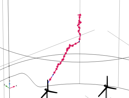
1
|
|
2
|
|
3
|
Clear the Plot dataset edges checkbox.
|
|
1
|
|
2
|
|
3
|
|
1
|
|
1
|
|
2
|
|
3
|
|
4
|
|
1
|
|
2
|
|
1
|
|
2
|
|
3
|
|
4
|
|
5
|
|
6
|
|
7
|
|
8
|
|
9
|
|
10
|
|
11
|
|
12
|
|
13
|
|
14
|
|
15
|
|
16
|
|
17
|
|
18
|
Click
|
|
1
|
|
3
|
|
4
|
|
5
|
Click to select the
|
|
6
|
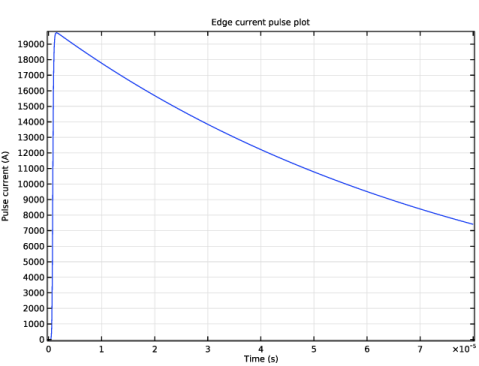
In the list, select 2385.
|
|
7
|
|
9
|
|
10
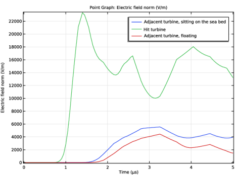
|
Select the Show legends checkbox.
|
|
11
|