
|
|
|


|
•
|
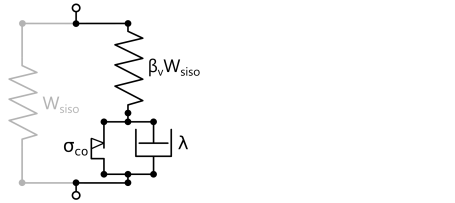
You can use the Bergstrom–Boyce material model by adding a Polymer Viscoplasticity node under Hyperelastic Material.
|
|
•
|
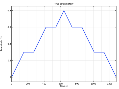
The desired true strain history can be imposed by applying a Predescribed Displacement node on the top surface of the specimen. The displacement can be computed as
|
|
•
|
You find the Domain ODEs option in the Time stepping section of the Polymer Viscoplasticity node. This option can be faster than Backward Euler when the number of degrees of freedom is small.
|
|
1
|
|
2
|
|
3
|
Click Add.
|
|
4
|
Click
|
|
5
|
|
6
|
Click
|
|
1
|
|
2
|
|
3
|
Locate the Parameters section. In the table, enter the following settings:
|
|
1
|
|
2
|
|
3
|
Locate the Parameters section. In the table, enter the following settings:
|
|
1
|
|
2
|
|
3
|
|
1
|
|
2
|
|
3
|
|
4
|
|
5
|
Click
|
|
6
|
Click
|
|
1
|
|
2
|
|
3
|
|
4
|
Find the Intervals subsection. In the table, enter the following settings:
|
|
5
|
|
6
|
|
7
|
Click
|
|
8
|
|
1
|
|
2
|
|
3
|
|
5
|
|
1
|
|
2
|
|
3
|
From the list, choose Quasistatic.
|
|
1
|
|
1
|
|
2
|
|
3
|
|
4
|
|
5
|
|
1
|
|
2
|
|
3
|
|
4
|
|
1
|
|
2
|
|
3
|
|
4
|
|
1
|
In the Model Builder window, under Component 1 (comp1) right-click Materials and choose Blank Material.
|
|
2
|
|
1
|
|
3
|
|
4
|
|
5
|
Click
|
|
1
|
|
2
|
|
3
|
|
1
|
|
2
|
|
3
|
|
1
|
|
2
|
|
3
|
In the Model Builder window, expand the Nonequilibrium Modeling > Solver Configurations > Solution 1 (sol1) > Time-Dependent Solver 1 node.
|
|
4
|
In the Model Builder window, expand the Nonequilibrium Modeling > Solver Configurations > Solution 1 (sol1) > Dependent Variables 1 node, then click Displacement Field (comp1.u).
|
|
5
|
|
6
|
|
7
|
In the Model Builder window, under Nonequilibrium Modeling > Solver Configurations > Solution 1 (sol1) > Dependent Variables 1 click Equivalent Viscoplastic Strain (comp1.solid.hmm1.pvp1.evpe).
|
|
8
|
|
9
|
|
10
|
In the Model Builder window, under Nonequilibrium Modeling > Solver Configurations > Solution 1 (sol1) > Dependent Variables 1 click Viscoplastic Strain Tensor, Local Coordinate System (comp1.solid.hmm1.pvp1.evp).
|
|
11
|
|
12
|
|
13
|
In the Model Builder window, under Nonequilibrium Modeling > Solver Configurations > Solution 1 (sol1) click Time-Dependent Solver 1.
|
|
14
|
|
15
|
|
16
|
|
1
|
|
2
|
|
3
|
Click
|
|
4
|
|
5
|
Click OK.
|
|
6
|
|
8
|
Select the Apply conversions to expressions with the same dimensions checkbox.
|
|
9
|
Click
|
|
1
|
|
2
|
|
1
|
|
2
|
|
3
|
|
1
|
|
2
|
|
3
|
|
4
|
|
5
|
|
6
|
|
1
|
|
2
|
|
3
|
|
1
|
|
2
|
|
3
|
|
1
|
|
2
|
|
1
|
|
2
|
|
3
|
|
4
|
|
5
|
Locate the Plot Settings section.
|
|
6
|
|
1
|
|
2
|
|
4
|
|
1
|
|
2
|
|
3
|
|
4
|
|
1
|
|
2
|
|
3
|
|
4
|
|
5
|
Locate the Plot Settings section.
|
|
6
|
|
7
|
|
1
|
|
2
|
|
4
|
|
5
|
|
6
|
|
7
|
|
1
|
|
2
|
|
3
|
|
1
|
|
2
|
|
3
|
|
4
|
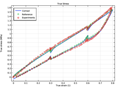
Browse to the model’s Application Libraries folder and double-click the file chloroprene_rubber_compression_test_numerical.txt.
|
|
1
|
|
2
|
|
3
|
|
4
|
|
5
|
|
6
|
|
1
|
|
2
|
|
3
|
|
4
|
Browse to the model’s Application Libraries folder and double-click the file chloroprene_rubber_compression_test_experimental.txt.
|
|
1
|
|
2
|
|
3
|
|
4
|
Locate the Coloring and Style section. Find the Line style subsection. From the Line list, choose None.
|
|
5
|
|
6
|
|
7
|
|
9
|
|
1
|
|
2
|
|
3
|
|
4
|
|
1
|
|
2
|
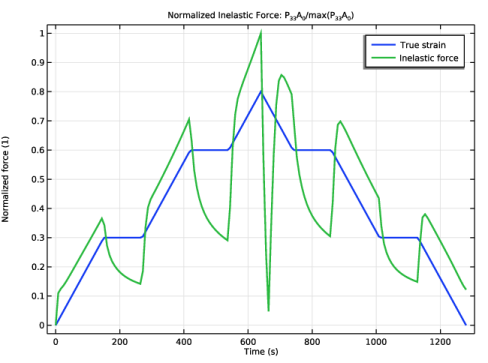
In the Settings window for 1D Plot Group, type Inelastic Force Contribution in the Label text field.
|
|
3
|
|
4
|
In the Title text area, type Normalized Inelastic Force: P<SUB>33</SUB>A<SUB>0</SUB>/max(P<SUB>33</SUB>A<SUB>0</SUB>).
|
|
5
|
Locate the Plot Settings section.
|
|
6
|
|
1
|
|
2
|
|
4
|
|
1
|
|
2
|
|
4
|
Locate the Expressions section. In the table, enter the following settings:
|
|
5
|
|
6
|
Click
|
|
1
|
|
2
|
|
4
|
|
1
|
|
2
|
Go to the Add Study window.
|
|
3
|
|
4
|
Click the Add Study button in the window toolbar.
|
|
5
|
|
1
|
|
2
|
|
1
|
|
2
|
|
3
|
|
4
|
Locate the Physics and Variables Selection section. Select the Modify model configuration for study step checkbox.
|
|
5
|
In the tree, select Component 1 (comp1) > Solid Mechanics (solid), Controls spatial frame > Hyperelastic Material 1 > Polymer Viscoplasticity 1.
|
|
6
|
Right-click and choose Disable.
|
|
1
|
|
2
|
|
3
|
|
4
|
|
5
|
In the Model Builder window, expand the Equilibrium Modeling > Solver Configurations > Solution 2 (sol2) > Time-Dependent Solver 1 node, then click Fully Coupled 1.
|
|
6
|
|
7
|
|
8
|
In the Model Builder window, expand the Equilibrium Modeling > Solver Configurations > Solution 2 (sol2) > Dependent Variables 1 node, then click Displacement Field (comp1.u).
|
|
9
|
|
10
|
|
11
|
|
1
|
|
2
|
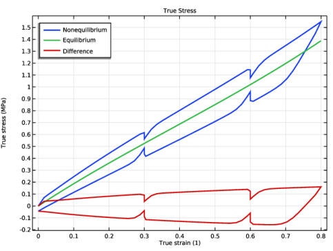
In the Settings window for 1D Plot Group, type Nonequilibrium vs. Equilibrium in the Label text field.
|
|
3
|
|
4
|
|
5
|
Locate the Plot Settings section.
|
|
6
|
|
7
|
|
8
|
|
1
|
|
2
|
|
3
|
Locate the y-Axis Data section. In the table, enter the following settings:
|
|
4
|
|
5
|
|
6
|
Clear the Solution checkbox.
|
|
7
|
Clear the Description checkbox.
|
|
8
|
|
9
|
|
1
|
|
2
|
|
3
|
|
1
|
|
2
|
|
3
|
Locate the y-Axis Data section. In the table, enter the following settings:
|
|
4
|