PDF

Two-Phase Flow in a Polymer Electrolyte Membrane Fuel Cell
Introduction
In a polymer electrolyte membrane fuel cell (PEMFC), water is produced at the cathode, and the cell is usually also fed with water vapor via the inlet gas streams.
This tutorial investigates the effects of water condensation in a polymer electrolyte membrane fuel cell with parallel flow channels.
In the model, condensation may result due to production of water at the cathode, but also due to the removal of other reactant species (H2 or O2) from the gas mixtures.
The resulting two-phase flow, fully coupled to the cell current distribution and mass transfer, is included in both the channels and the gas diffusion layers.
Model Definition
Figure 1: Model geometry.
Figure 1 shows the full model geometry. The cell geometry consists of two parallel flow channels on each side of the membrane-electrode-assembly (MEA). The MEA is defined as three rectangular block domains defining the hydrogen-side gas diffusion layer (GDL), the membrane and the oxygen-side GDL.
The model is setup using the Hydrogen Fuel Cell interface together with the Free and Porous Multiphase Flow multiphysics interface.
Volume Fractions
The Phase Transport in Free and Porous Media Flow interface solves for the relative liquid water volume fraction sw in the gas pores in the GDLs and the channels. The relative gas volume fraction is then defined as
As liquid water condenses in the GDLs and is transported out to the channels, the volume fraction of gas decreases, making room for the produced liquid.
In the GDLs, the gas volume fraction εg is defined as
where εpor is the pore volume fraction relative to the total volume.
Hydrogen Fuel Cell Interface
The current distribution, electrochemical and water condensation-evaporation reactions are defined using the Hydrogen Fuel Cell interface. The gas diffusion electrode reactions are modeled using Butler–Volmer kinetics. Ohmic losses in the electrode and electrolyte phases are included. Electroosmotic water drag is enabled in the model, allowing for membrane transport of water between the oxygen and hydrogen compartment.
The fuel cell part of the model is very similar to the Low-Temperature PEM Fuel Cell with Serpentine Flow Field tutorial and more details about the setup of the Hydrogen Fuel Cell interface can be found in this example.
Gas diffusion in relation to the mass-averaged gas-phase velocity is defined by the fuel cell interface, solving for the mass fractions of the gas species in the gas mixtures, whereas the mass-averaged velocity and pressure are defined by the Darcy’s Law and Laminar Flow interfaces (see below).
The effective gas diffusivities in the GDLs on each side of the membrane is set to depend on the electrolyte volume fraction according to
(1)
where Dij are the binary (bulk) diffusivities of the gas species.
In the channels, the water volume fraction is assumed to be so low that the impact on the gas diffusivity may be neglected.
An average cell current density of 1 A/cm2 is applied on the cathode current conductor.
The cell fed with humidified air and hydrogen mixtures, humidified to 100% relative humidity (RH).
Multiphase Flow In Free and Porous Media Multiphysics Interface
The two-phase flow model is defined by adding a Multiphase Flow in Free and Porous Media multiphysics interface to the model. This in turn adds the following physics interfaces to the model tree:
Darcy’s Law, solving for the pressure in the GDLs
Laminar Flow, solving for the gas pressure and velocity field in the channels
Phase Transport in Free and Porous Media Flow, solving for the liquid water phase volume fraction in the gas-liquid two-phase mixture
In addition, the following multiphysics nodes are also added by Multiphase Flow in Free and Porous Media:
Multiphase Flow in Porous Media, coupling Darcy’s law and Phase Transport in the GDLs
Free and Porous Media Flow Coupling, defining the boundary between the Laminar Flow and Darcy’s Law domains
Mixture Model, coupling Laminar Flow and Phase Transport in the channels
The gas and liquid mass sources, stemming from the electrode reactions defined by the Hydrogen Fuel Cell interface, are added as a Mass Source node in the Phase Transport in Free and Porous Media Flow interface. Turbulent Mixing is added in the channels in the Phase Transport in Free and Porous Media Flow interface in order to facilitate convergence.
Fully-developed flow conditions are defined on the Inlet nodes in the Laminar Flow interface, specifying mass flow rates corresponding to a hydrogen and oxygen stoichiometry of 2 and 2.5, respectively. A uniform absolute outlet pressure of 1 atm is defined on the Outlet node in the same interface.
Capillary Pressure and Residual Saturation
In the GDLs, the liquid water transport will be governed by the capillary pressure and the relative permeabilities of the two phases, both being functions of the water saturation level as defined on the Porous Medium>Fluid node of the Phase Transport in Free and Porous Media Flow interface. In this tutorial, the Brooks and Corey model is used, using parameters found in Ref. 1.
The residual saturation, srs (dimensionless), defines the amount of liquid water remaining in the porous structure at zero capillary pressure. One reason for the remaining water is the formation of a thin water film on the pore wall surfaces within the matrix, also at relative humidities below 100%. Assuming the film thickness to scale linearly with the relative humidity, we use the following relation between the relative humidity and the residual saturation
(2)
where srs, 100% RH is the residual saturation at 100% relative humidity, and RH is the relative humidity, regularized between 0 and 100%.
The variable srs is used both in the Brooks and Corey model for the capillary pressure and permeabilities, and as a boundary condition for setting the liquid saturation level at the GDL-channel boundaries.
Water Condensation and Evaporation
Due to the significantly larger internal surface area of the GDLs in comparison to the channels, water is assumed to condensate or evaporate in the GDL domains only.
The rate expression for water condensation is defined as
(3)
where kw is a rate constant and aH2O(g) and aH2O(l) are the thermodynamic activities of water in the gas and liquid phases, respectively.
The gas phase thermodynamic activity is related to the partial pressure of gaseous water as
(4)
whereas the thermodynamic liquid water activity is related to the water vapor pressure as
(5)
for the case when the liquid saturation level is higher than the residual saturation at 100% RH (sw > srs, 100% RH). When the liquid saturation is lower than the residual saturation (sw < srs, 100% RH) at 100% RH, the liquid water activity is defined as
(6)
Study
Four consecutive study steps are used to solve the model. For each step, the solution of the dependent variables solved for in the previous step are passed on as the corresponding initial values to the subsequent step.
A first Current Distribution Initialization step computes suitable initial values for the electrode and electrolyte phase potentials, neglecting nonlinear activation overpotentials.
The second Current Distribution Initialization step includes nonlinear activation overpotentials.
A third Stationary step then solves for the pressures and velocity fields of the Darcy’s Law and Laminar Flow interfaces only, with all resulting mass sources from the fuel cell model disabled.
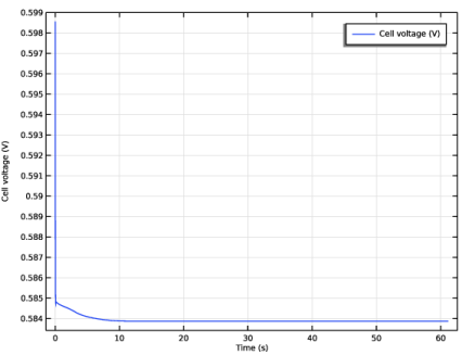
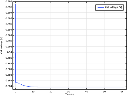
The fourth and final Time Dependent step solves for the fully coupled problem using a time-dependent solver, representing the transient behavior of the cell during 60 s after a current step going from a 0 to 1 A/cm2 average cell current density at t = 0 s.
Results and Discussion
Figure 2 shows the cell voltage versus time. The lowered cell voltage over time is due to a lowered oxygen partial pressure at the cathode. It takes about 10 s before a steady-state voltage establishes.
Figure 3 shows the cross-membrane current density at the end of the simulation. The current density decreases toward the outlet. As we will see, this is also related to the oxygen partial pressure.
Figure 2: Cell voltage versus time.
Figure 3: Cross-membrane current density.
Figure 4 and Figure 5 show the hydrogen and oxygen molar fractions in the cell at the end of the simulation, respectively.
The hydrogen molar fraction is more or less uniform in Figure 4. This is a result of continuous condensation of water as hydrogen is oxidized and removed from the fuel stream, maintaining a relative humidity close to 100%.
The oxygen molar fraction in Figure 5 on the other hand decreases gradually toward the outlet. Also here the relative humidity remains close to 100%, but as oxygen is reduced and removed from the oxidant stream, the molar fraction of nitrogen increases.
Figure 4: Hydrogen molar fraction.
Figure 5: Oxygen molar fraction.
Figure 6 shows the velocity magnitude in the channels. On the oxygen side, the velocity magnitude decreases slightly toward the outlet. This results from oxygen being removed from the gaseous oxidant stream. However, since the relative molar fraction of oxygen is relatively low, the relative velocity decrease is limited. On the hydrogen side, the velocity decrease is more significant.
Finally, the liquid water volume fraction in the GDLs and channels are shown in Figure 7. The liquid water volume fraction is generally low in the channels, this is directly related to the orders of magnitudes larger density of the liquid phase.
The volume fraction increases slightly toward the outlet side, and interestingly it is slightly higher in the hydrogen channels, compared to the oxygen side. This is a result of the relatively larger volumetric utilization of hydrogen gas stream.
Figure 6: Velocity magnitude in channels.
Figure 7: Liquid volume fraction.
Reference
1. N. Zamel, X. Li, J. Becker, and A. Wiegmann, “Effect of liquid water on transport properties of the gas diffusion layer of polymer electrolyte membrane fuel cells,” Int. J. Hydrogen Energy, vol. 36, no. 9, pp. 5466–5478, 2011.
Application Library path: Fuel_Cell_and_Electrolyzer_Module/Fuel_Cells/two_phase_pemfc
Modeling Instructions
From the File menu, choose New.
New
In the New window, click  Model Wizard.
Model Wizard
1
In the Model Wizard window, click  3D.
2
In the Select Physics tree, select Electrochemistry > Hydrogen Fuel Cells > Proton Exchange Membrane (fc).
3
Click Add.
4
In the Select Physics tree, select Fluid Flow > Porous Media and Subsurface Flow > Multiphase Free and Porous Media Flow.
5
Click Add.
6
In the Added physics interfaces tree, select Phase Transport in Free and Porous Media Flow (phtr).
7
In the Volume fractions (1) table, enter the following settings:
8
Click  Study.
9
In the Select Study tree, select Preset Studies for Selected Physics Interfaces > Hydrogen Fuel Cell > Time Dependent with Initialization.
10
Geometry 1
1
In the Geometry toolbar, click Insert Sequence and choose Insert Sequence.
2
3
In the Model Builder window, under Component 1 (comp1) click Geometry 1.
4
In the Model Builder window, collapse the Geometry 1 node.
Global Definitions
Geometry Parameters
1
In the Model Builder window, under Global Definitions click Parameters 1.
2
In the Settings window for Parameters, type Geometry Parameters in the Label text field.
Physics Parameters
1
In the Home toolbar, click  Parameters and choose Add > Parameters.
2
In the Settings window for Parameters, type Physics Parameters in the Label text field.
3
Locate the Parameters section. Click  Load from File.
4
Definitions
GDL Variables
1
In the Model Builder window, under Component 1 (comp1) right-click Definitions and choose Variables.
2
In the Settings window for Variables, type GDL Variables in the Label text field.
3
Locate the Geometric Entity Selection section. From the Geometric entity level list, choose Domain.
4
From the Selection list, choose GDLs.
5
Locate the Variables section. Click  Load from File.
6
Channel Variables
1
In the Model Builder window, right-click Definitions and choose Variables.
2
In the Settings window for Variables, type Channel Variables in the Label text field.
3
Locate the Geometric Entity Selection section. From the Geometric entity level list, choose Domain.
4
From the Selection list, choose Channels.
5
Locate the Variables section. Click  Load from File.
6
The two variable nodes you just added define the absolute pressure (pA) and velocity (U/V/W) differently in the channels and gdls, respectively. These variables will be used to define the gas phase properties in the Hydrogen Fuel Cell interface.
Add Material
1
In the Materials toolbar, click  Add Material to open the Add Material window.
2
Go to the Add Material window.
3
In the tree, select Fuel Cell and Electrolyzer > Polymer Electrolytes > Nafion®, EW 1100, Vapor Equilibrated, Protonated.
4
Right-click and choose Add to Component 1 (comp1).
5
In the Materials toolbar, click  Add Material to close the Add Material window.
Materials
Nafion®, EW 1100, Vapor Equilibrated, Protonated (mat1)
1
In the Settings window for Material, locate the Geometric Entity Selection section.
2
From the Selection list, choose Membrane.
Nafion®, EW 1100, Vapor Equilibrated, Protonated 1 (mat2)
1
Right-click Component 1 (comp1) > Materials > Nafion®, EW 1100, Vapor Equilibrated, Protonated (mat1) and choose Duplicate.
Two instances of the Nafion material is required for this model. The domain node defines the transport properties (such as conductivity) of the membrane, and the boundary node defines the water adsorption-desorption properties between the membrane and the gas phase.
2
In the Settings window for Material, locate the Geometric Entity Selection section.
3
From the Geometric entity level list, choose Boundary.
4
From the Selection list, choose GDEs.
Hydrogen Fuel Cell (fc)
1
In the Model Builder window, under Component 1 (comp1) click Hydrogen Fuel Cell (fc).
2
In the Settings window for Hydrogen Fuel Cell, locate the H2 Gas Mixture section.
3
Find the Reactions subsection. Select the Include H2O(l) in reaction stoichiometry checkbox.
4
Locate the O2 Gas Mixture section. Select the Include H2O(l) in reaction stoichiometry checkbox.
Enabling the above checkboxes allows for defining rate expressions for liquid water due to evaporation-condensation.
5
Click to expand the Membrane Transport section. Select the Electroosmotic water drag checkbox.
Membrane 1
1
In the Physics toolbar, click  Domains and choose Membrane.
2
In the Settings window for Membrane, locate the Domain Selection section.
3
From the Selection list, choose Membrane.
Initial Values 1
1
In the Model Builder window, expand the Membrane 1 node, then click Initial Values 1.
2
In the Settings window for Initial Values, locate the Initial Values section.
3
In the aw,0 text field, type RH.
4
In the T0 text field, type T.
Hydrogen Fuel Cell (fc)
Membrane 1
In the Model Builder window, collapse the Component 1 (comp1) > Hydrogen Fuel Cell (fc) > Membrane 1 node.
H2 Gas Diffusion Layer 1
1
In the Physics toolbar, click  Domains and choose H2 Gas Diffusion Layer.
2
In the Settings window for H2 Gas Diffusion Layer, locate the Domain Selection section.
3
From the Selection list, choose Hydrogen GDL.
4
Locate the Electrode Charge Transport section. From the list, choose Diagonal.
5
Specify the σs matrix as
6
Locate the Gas Transport section. In the εg text field, type epsg_gdl.
O2 Gas Diffusion Layer 1
1
In the Physics toolbar, click  Domains and choose O2 Gas Diffusion Layer.
2
In the Settings window for O2 Gas Diffusion Layer, locate the Domain Selection section.
3
From the Selection list, choose Oxygen GDL.
4
Locate the Electrode Charge Transport section. From the list, choose Diagonal.
5
Specify the σs matrix as
6
Locate the Gas Transport section. In the εg text field, type epsg_gdl.
Thin H2 Gas Diffusion Electrode 1
1
In the Physics toolbar, click  Boundaries and choose Thin H2 Gas Diffusion Electrode.
2
In the Settings window for Thin H2 Gas Diffusion Electrode, locate the Boundary Selection section.
3
From the Selection list, choose Hydrogen GDE.
4
Locate the Electrode Thickness section. In the dgde text field, type H_cl.
Thin H2 Gas Diffusion Electrode Reaction 1
1
In the Model Builder window, click Thin H2 Gas Diffusion Electrode Reaction 1.
2
In the Settings window for Thin H2 Gas Diffusion Electrode Reaction, locate the Electrode Kinetics section.
3
In the i0,ref(T) text field, type i0_ref_HOR.
4
Locate the Active Specific Surface Area section. In the av text field, type Av_HOR.
Thin O2 Gas Diffusion Electrode 1
1
In the Physics toolbar, click  Boundaries and choose Thin O2 Gas Diffusion Electrode.
2
In the Settings window for Thin O2 Gas Diffusion Electrode, locate the Boundary Selection section.
3
From the Selection list, choose Oxygen GDE.
4
Locate the Electrode Thickness section. In the dgde text field, type H_cl.
Thin O2 Gas Diffusion Electrode Reaction 1
1
In the Model Builder window, click Thin O2 Gas Diffusion Electrode Reaction 1.
2
In the Settings window for Thin O2 Gas Diffusion Electrode Reaction, locate the Electrode Kinetics section.
3
In the i0,ref(T) text field, type i0_ref_ORR.
4
In the αa text field, type alphaa_ORR.
5
Locate the Active Specific Surface Area section. In the av text field, type Av_ORR.
H2 Gas Flow Channel 1
1
In the Physics toolbar, click  Domains and choose H2 Gas Flow Channel.
2
In the Settings window for H2 Gas Flow Channel, locate the Domain Selection section.
3
From the Selection list, choose Hydrogen Channels.
O2 Gas Flow Channel 1
1
In the Physics toolbar, click  Domains and choose O2 Gas Flow Channel.
2
In the Settings window for O2 Gas Flow Channel, locate the Domain Selection section.
3
From the Selection list, choose Oxygen Channels.
Electronic Conducting Phase 1
In the Model Builder window, click Electronic Conducting Phase 1.
Electric Ground 1
1
In the Physics toolbar, click  Attributes and choose Electric Ground.
2
In the Settings window for Electric Ground, locate the Boundary Selection section.
3
From the Selection list, choose Anode Current Collector.
Electronic Conducting Phase 1
In the Model Builder window, click Electronic Conducting Phase 1.
Electrode Current 1
1
In the Physics toolbar, click  Attributes and choose Electrode Current.
2
In the Settings window for Electrode Current, locate the Electrode Current section.
3
In the Is,total text field, type -I_cell.
4
Locate the Boundary Selection section. From the Selection list, choose Cathode Current Collector.
H2 Gas Phase 1
1
In the Model Builder window, under Component 1 (comp1) > Hydrogen Fuel Cell (fc) click H2 Gas Phase 1.
2
In the Settings window for H2 Gas Phase, locate the Model Input section.
3
From the pA list, choose User defined. In the associated text field, type pA.
4
Locate the Convection section. Specify the u vector as
H2 Inlet 1
1
In the Physics toolbar, click  Attributes and choose H2 Inlet.
2
In the Settings window for H2 Inlet, locate the Boundary Selection section.
3
From the Selection list, choose Hydrogen Inlets.
H2 Gas Phase 1
In the Model Builder window, click H2 Gas Phase 1.
H2 Outlet 1
1
In the Physics toolbar, click  Attributes and choose H2 Outlet.
2
In the Settings window for H2 Outlet, locate the Boundary Selection section.
3
From the Selection list, choose Hydrogen Outlets.
H2 Gas Phase 1
In the Model Builder window, click H2 Gas Phase 1.
Water Condensation-Evaporation 1
1
In the Physics toolbar, click  Attributes and choose Water Condensation-Evaporation.
2
In the Settings window for Water Condensation-Evaporation, locate the Domain Selection section.
3
From the Selection list, choose Hydrogen GDL.
4
Locate the Condensation-Evaporation Rate section. From the rce list, choose User defined. In the text field, type r_c.
Initial Values 1
1
In the Model Builder window, click Initial Values 1.
2
In the Settings window for Initial Values, locate the Initial Composition section.
3
From the Mixture specification list, choose Humidified mixture.
4
In the RHhum text field, type RH.
5
In the Thum text field, type T.
O2 Gas Phase 1
1
In the Model Builder window, under Component 1 (comp1) > Hydrogen Fuel Cell (fc) click O2 Gas Phase 1.
2
In the Settings window for O2 Gas Phase, locate the Model Input section.
3
From the pA list, choose User defined. In the associated text field, type pA.
4
Locate the Convection section. Specify the u vector as
O2 Inlet 1
1
In the Physics toolbar, click  Attributes and choose O2 Inlet.
2
In the Settings window for O2 Inlet, locate the Boundary Selection section.
3
From the Selection list, choose Oxygen Inlets.
O2 Gas Phase 1
In the Model Builder window, click O2 Gas Phase 1.
O2 Outlet 1
1
In the Physics toolbar, click  Attributes and choose O2 Outlet.
2
In the Settings window for O2 Outlet, locate the Boundary Selection section.
3
From the Selection list, choose Oxygen Outlets.
O2 Gas Phase 1
In the Model Builder window, click O2 Gas Phase 1.
Water Condensation-Evaporation 1
1
In the Physics toolbar, click  Attributes and choose Water Condensation-Evaporation.
2
In the Settings window for Water Condensation-Evaporation, locate the Domain Selection section.
3
From the Selection list, choose Oxygen GDL.
4
Locate the Condensation-Evaporation Rate section. From the rce list, choose User defined. In the text field, type r_c.
Initial Values 1
1
In the Model Builder window, click Initial Values 1.
2
In the Settings window for Initial Values, locate the Initial Composition section.
3
From the Mixture specification list, choose Humidified air.
4
In the RHhum text field, type RH.
5
In the Thum text field, type T.
Hydrogen Fuel Cell (fc)
In the Model Builder window, collapse the Component 1 (comp1) > Hydrogen Fuel Cell (fc) node.
Laminar Flow (spf)
The settings of the fuel cell interface are now complete. Proceed to set up the conditions for the flow in the channels.
1
In the Model Builder window, under Component 1 (comp1) click Laminar Flow (spf).
2
In the Settings window for Laminar Flow, locate the Domain Selection section.
3
From the Selection list, choose Channels.
Inlet 1
1
In the Physics toolbar, click  Boundaries and choose Inlet.
2
In the Settings window for Inlet, locate the Boundary Selection section.
3
From the Selection list, choose Oxygen Inlets.
4
Locate the Boundary Condition section. From the list, choose Mass flow.
5
Clear the Apply condition on each disjoint selection separately checkbox.
Disabling the above checkbox means that a common pressure will be applied on all inlet boundaries. The pressure will be set so that it fulfills the total mass flow M_cath specified.
6
Locate the Mass Flow section. In the m text field, type M_cath.
Inlet 2
1
In the Physics toolbar, click  Boundaries and choose Inlet.
2
In the Settings window for Inlet, locate the Boundary Selection section.
3
From the Selection list, choose Hydrogen Inlets.
4
Locate the Boundary Condition section. From the list, choose Mass flow.
5
Clear the Apply condition on each disjoint selection separately checkbox.
6
Locate the Mass Flow section. In the m text field, type M_an.
Outlet 1
1
In the Physics toolbar, click  Boundaries and choose Outlet.
2
In the Settings window for Outlet, locate the Boundary Selection section.
3
From the Selection list, choose Outlets.
Laminar Flow (spf)
In the Model Builder window, collapse the Component 1 (comp1) > Laminar Flow (spf) node.
Darcy’s Law (dl)
Darcy’s law is used in this model to define the pressure and velocity field in the gdls.
1
In the Model Builder window, under Component 1 (comp1) click Darcy’s Law (dl).
2
In the Settings window for Darcy’s Law, locate the Domain Selection section.
3
From the Selection list, choose GDLs.
Porous Matrix 1
1
In the Model Builder window, under Component 1 (comp1) > Darcy’s Law (dl) > Porous Medium 1 click Porous Matrix 1.
2
In the Settings window for Porous Matrix, locate the Matrix Properties section.
3
From the εp list, choose User defined. In the associated text field, type por_gdl.
4
From the κ list, choose User defined. In the associated text field, type perm_gdl.
5
In the Model Builder window, collapse the Darcy’s Law (dl) node.
Phase Transport in Free and Porous Media Flow (phtr)
The phase transport model solves for the volume fraction of liquid water in the channels and the gdls.
1
In the Model Builder window, under Component 1 (comp1) click Phase Transport in Free and Porous Media Flow (phtr).
2
In the Settings window for Phase Transport in Free and Porous Media Flow, locate the Domain Selection section.
3
From the Selection list, choose Flow Domains.
Fluid 1
In the Model Builder window, under Component 1 (comp1) > Phase Transport in Free and Porous Media Flow (phtr) click Fluid 1.
Turbulent Mixing 1
1
In the Physics toolbar, click  Attributes and choose Turbulent Mixing.
2
In the Settings window for Turbulent Mixing, locate the Turbulent Mixing Parameters section.
3
In the νT text field, type D_eddy.
4
In the ScT text field, type 1.
Porous Medium 1
1
In the Model Builder window, under Component 1 (comp1) > Phase Transport in Free and Porous Media Flow (phtr) click Porous Medium 1.
2
In the Settings window for Porous Medium, locate the Domain Selection section.
3
From the Selection list, choose GDLs.
Fluid 1
1
In the Model Builder window, click Fluid 1.
2
In the Settings window for Fluid, locate the Capillary Pressure section.
3
From the Capillary pressure model list, choose Brooks and Corey.
4
In the pec text field, type p_BC.
5
In the λp text field, type lambda_BC.
6
Locate the Phase 1 Properties section. From the ρsg list, choose Density of gas phase (fc).
7
From the μsg list, choose Dynamic viscosity of gas phase (fc).
8
Locate the Phase 2 Properties section. From the ρsw list, choose Density of liquid water (fc).
9
From the μsw list, choose Dynamic viscosity of liquid water (fc).
10
In the srsw text field, type sw_res.
Initial Values - GDLs
1
In the Physics toolbar, click  Domains and choose Initial Values.
2
In the Settings window for Initial Values, type Initial Values - GDLs in the Label text field.
3
Locate the Domain Selection section. From the Selection list, choose GDLs.
4
Locate the Initial Values section. In the s0,sw text field, type sw_res_100_aw*RH.
Volume Fraction 1
1
In the Physics toolbar, click  Boundaries and choose Volume Fraction.
2
In the Settings window for Volume Fraction, locate the Boundary Selection section.
3
From the Selection list, choose Inlets.
4
Locate the Volume Fraction section. Select the Phase s_w checkbox.
Outflow 1
1
In the Physics toolbar, click  Boundaries and choose Outflow.
2
In the Settings window for Outflow, locate the Boundary Selection section.
3
From the Selection list, choose Outlets.
Mass Source 1
Use a Mass Source node to add the gas and liquid phase mass sources defined by the Hydrogen Fuel Cell interface.
By enabling the Mass transfer to other phases checkbox, the net mass source (or sink) will also be added to the Darcy’s law interface via the Multiphase Flow in Porous Media multiphysics node.
1
In the Physics toolbar, click  Domains and choose Mass Source.
2
In the Settings window for Mass Source, locate the Domain Selection section.
3
From the Selection list, choose GDLs.
4
Locate the Mass Source section. Select the Mass transfer to other phases checkbox.
5
From the Qsg list, choose Mass source, gas phase (fc).
6
From the Qsw list, choose Mass source, liquid phase (fc).
Boundary Mass Source 1
Use a Boundary Mass Source node to add the gas and liquid phase mass sources defined by the Hydrogen Fuel Cell interface.
1
In the Physics toolbar, click  Boundaries and choose Boundary Mass Source.
2
In the Settings window for Boundary Mass Source, locate the Boundary Selection section.
3
From the Selection list, choose GDEs.
4
Locate the Boundary Mass Source section. From the qb,sg list, choose Boundary mass source, gas phase (fc).
5
From the qb,sw list, choose Boundary mass source, liquid phase (fc).
Phase Transport in Free and Porous Media Flow (phtr)
In the Model Builder window, collapse the Component 1 (comp1) > Phase Transport in Free and Porous Media Flow (phtr) node.
Multiphysics
Mixture Model 1 (mfmm1)
The mixture model defines the two-phase properties in the channels.
1
In the Model Builder window, under Component 1 (comp1) > Multiphysics click Mixture Model 1 (mfmm1).
2
In the Settings window for Mixture Model, locate the Physical Model section.
3
From the Dispersed phase list, choose Liquid droplets/bubbles.
4
Locate the Continuous Phase Properties section. From the ρc list, choose Density of gas phase (fc).
5
From the μc list, choose Dynamic viscosity of gas phase (fc).
6
Locate the Dispersed Phase 2 Properties section. From the ρsw list, choose Density of liquid water (fc).
7
From the μsw list, choose Dynamic viscosity of liquid water (fc).
Global Definitions
Default Model Inputs
Define the temperature on the Default Model Inputs node in order to use the same temperature setting on all nodes in the model.
1
In the Model Builder window, under Global Definitions click Default Model Inputs.
2
In the Settings window for Default Model Inputs, locate the Browse Model Inputs section.
3
In the tree, select General > Temperature (K) - minput.T.
4
Find the Expression for remaining selection subsection. In the Temperature text field, type T.
Multiphysics
In the Model Builder window, collapse the Component 1 (comp1) > Multiphysics node.
Mesh 1
The physics settings are now complete. Now create a mesh by sweeping the oxygen channels first, then through the GDLs and membrane, and finally the hydrogen channels.
1
In the Model Builder window, under Component 1 (comp1) click Mesh 1.
2
In the Settings window for Mesh, locate the Sequence Type section.
3
From the list, choose User-controlled mesh.
4
In the Mesh toolbar, click  Clear Sequence.
Mapped 1
1
In the Mesh toolbar, click  More Generators and choose Mapped.
2
In the Settings window for Mapped, locate the Boundary Selection section.
3
From the Selection list, choose Inlets.
Distribution 1
1
Right-click Mapped 1 and choose Distribution.
2
In the Settings window for Distribution, locate the Edge Selection section.
3
From the Selection list, choose All edges.
4
Locate the Distribution section. From the Distribution type list, choose Predefined.
5
In the Number of elements text field, type 8.
6
In the Element ratio text field, type 2.
7
Select the Symmetric distribution checkbox.
Swept 1
1
In the Mesh toolbar, click  Swept.
2
In the Settings window for Swept, locate the Domain Selection section.
3
From the Geometric entity level list, choose Domain.
4
From the Selection list, choose Oxygen Channels.
Size 1
1
Right-click Swept 1 and choose Size.
2
In the Settings window for Size, locate the Element Size section.
3
Click the Custom button.
4
Locate the Element Size Parameters section.
5
Select the Maximum element size checkbox. In the associated text field, type W_ribch.
Size 2
1
In the Model Builder window, right-click Swept 1 and choose Size.
2
In the Settings window for Size, locate the Geometric Entity Selection section.
3
From the Selection list, choose Bends.
4
Locate the Element Size section. Click the Custom button.
5
Locate the Element Size Parameters section.
6
Select the Maximum element size checkbox. In the associated text field, type H_ch/3.
Swept 1
1
Right-click Swept 1 and choose Build Selected.
2
Click the  Show Axis Orientation button in the Graphics toolbar.
3
Click the  Show Grid button in the Graphics toolbar.
4
Click the  Zoom Extents button in the Graphics toolbar.
Mapped 2
1
In the Mesh toolbar, click  More Generators and choose Mapped.
2
In the Settings window for Mapped, locate the Boundary Selection section.
3
From the Selection list, choose Cathode Current Collector.
Size 1
1
Right-click Mapped 2 and choose Size.
2
In the Settings window for Size, locate the Element Size section.
3
Click the Custom button.
4
Locate the Element Size Parameters section.
5
Select the Maximum element size checkbox. In the associated text field, type W_rib/10.
Mapped 2
In the Model Builder window, right-click Mapped 2 and choose Build Selected.
Copy Face 1
1
In the Mesh toolbar, click  Copy and choose Copy Face.
2
In the Settings window for Copy Face, locate the Source Boundaries section.
3
From the Selection list, choose Oxygen GDL Top Boundaries.
4
Locate the Destination Boundaries section. From the Selection list, choose Hydrogen GDL Bottom Boundaries.
5
Click  Build Selected.
Swept 2
1
In the Mesh toolbar, click  Swept.
2
In the Settings window for Swept, locate the Domain Selection section.
3
From the Geometric entity level list, choose Domain.
4
Distribution 1
1
Right-click Swept 2 and choose Distribution.
2
In the Settings window for Distribution, locate the Domain Selection section.
3
From the Selection list, choose GDLs.
4
Locate the Distribution section. From the Distribution type list, choose Predefined.
5
In the Number of elements text field, type 10.
6
In the Element ratio text field, type 3.
7
Select the Reverse direction checkbox.
Distribution 2
1
In the Model Builder window, right-click Swept 2 and choose Distribution.
2
In the Settings window for Distribution, locate the Domain Selection section.
3
From the Selection list, choose Membrane.
4
Locate the Distribution section. In the Number of elements text field, type 4.
Swept 2
Right-click Swept 2 and choose Build Selected.
Swept 3
1
In the Mesh toolbar, click  Swept.
2
In the Settings window for Swept, locate the Domain Selection section.
3
From the Geometric entity level list, choose Domain.
4
From the Selection list, choose Hydrogen Channels.
5
Click to expand the Source Faces section. From the Selection list, choose Hydrogen Inlets.
6
Click to expand the Destination Faces section. From the Selection list, choose Hydrogen Outlets.
Size 1
1
Right-click Swept 3 and choose Size.
2
In the Settings window for Size, locate the Element Size section.
3
Click the Custom button.
4
Locate the Element Size Parameters section.
5
Select the Maximum element size checkbox. In the associated text field, type W_ribch.
Size 2
1
In the Model Builder window, right-click Swept 3 and choose Size.
2
In the Settings window for Size, locate the Geometric Entity Selection section.
3
From the Selection list, choose Bends.
4
Locate the Element Size section. Click the Custom button.
5
Locate the Element Size Parameters section.
6
Select the Maximum element size checkbox. In the associated text field, type H_ch/3.
7
In the Model Builder window, right-click Mesh 1 and choose Build All.
Study 1
The physics and mesh are now complete. Modify the predefined study sequence by adding a second Current Distribution step and a Stationary step.
Each study step uses the results of the previous step as initial values. The Current Distribution step solves for a stationary current distribution for the initial gas distribution. By setting the distribution type to Secondary in the second step, nonlinear kinetics are included.
The additional Stationary step will be defined to solve for the single-phase (gas-only) initial flow distribution, setting all mass sources in the fuel cell to zero.
The final time-dependent step solves for the resulting transient flow changes when the average cell current density is changed from 0 to 1 A/cm2 at t = 0.
Step 3: Current Distribution Initialization 2
1
In the Study toolbar, click  Study Steps and choose Other > Current Distribution Initialization.
2
Right-click Step 3: Current Distribution Initialization 2 and choose Move Up.
3
In the Settings window for Current Distribution Initialization, locate the Study Settings section.
4
From the Current distribution type list, choose Secondary.
Stationary - Single Phase Flow Initialization
1
In the Study toolbar, click  Study Steps and choose Stationary > Stationary.
2
Right-click Step 4: Stationary and choose Move Up.
3
In the Settings window for Stationary, type Stationary - Single Phase Flow Initialization in the Label text field.
4
Locate the Physics and Variables Selection section. In the Solve for column of the table, under Component 1 (comp1), clear the checkboxes for Hydrogen Fuel Cell (fc) and Phase Transport in Free and Porous Media Flow (phtr).
5
Select the Modify model configuration for study step checkbox.
6
In the tree, select Component 1 (comp1) > Phase Transport in Free and Porous Media Flow (phtr) > Mass Source 1.
7
8
In the tree, select Component 1 (comp1) > Phase Transport in Free and Porous Media Flow (phtr) > Boundary Mass Source 1.
9
Step 4: Time Dependent
1
In the Model Builder window, click Step 4: Time Dependent.
2
In the Settings window for Time Dependent, locate the Study Settings section.
3
In the Output times text field, type 0 1 10 60.
Before solving, add a probe to monitor the cell voltage versus time for all time-steps taken by the solver.
Definitions
Global Variable Probe 1 (var1)
1
In the Definitions toolbar, click  Probes and choose Global Variable Probe.
2
In the Settings window for Global Variable Probe, click Replace Expression in the upper-right corner of the Expression section. From the menu, choose Component 1 (comp1) > Hydrogen Fuel Cell > fc.phis0_ec1 - Electric potential on boundary - V.
3
Locate the Expression section.
4
Select the Description checkbox. In the associated text field, type Cell voltage.
Study 1
Step 3: Stationary - Single Phase Flow Initialization
Probes are automatically disabled in the Current Distribution Initialization steps. Disable the probe in step 3 as follows:
1
In the Model Builder window, under Study 1 click Step 3: Stationary - Single Phase Flow Initialization.
2
In the Settings window for Stationary, click to expand the Results While Solving section.
3
From the Probes list, choose None.
The model is now ready for solving.
4
In the Study toolbar, click  Compute.
Results
Cell Voltage vs. Time
1
In the Model Builder window, under Results click Probe Plot Group 1.
2
In the Settings window for 1D Plot Group, type Cell Voltage vs. Time in the Label text field.
Mole Fraction, H2, Surface (fc)
1
In the Model Builder window, click Mole Fraction, H2, Surface (fc).
2
In the Settings window for 3D Plot Group, locate the Plot Settings section.
3
Clear the Plot dataset edges checkbox.
4
In the Mole Fraction, H2, Surface (fc) toolbar, click  Plot.
Mole Fraction, O2, Surface (fc)
1
In the Model Builder window, click Mole Fraction, O2, Surface (fc).
2
In the Settings window for 3D Plot Group, locate the Plot Settings section.
3
Clear the Plot dataset edges checkbox.
Slice
1
In the Model Builder window, expand the Velocity (spf) node, then click Slice.
2
In the Settings window for Slice, locate the Plane Data section.
3
From the Plane list, choose xy-planes.
4
From the Entry method list, choose Coordinates.
5
In the z-coordinates text field, type H_ch/2+H_mem/2+H_gdl.
Slice 2
1
Right-click Slice and choose Duplicate.
2
In the Settings window for Slice, click to expand the Title section.
3
From the Title type list, choose None.
4
Locate the Plane Data section. In the z-coordinates text field, type -(H_ch/2+H_mem/2+H_gdl).
5
Locate the Coloring and Style section. From the Color table list, choose Prism.
Velocity (spf)
1
In the Model Builder window, click Velocity (spf).
2
In the Settings window for 3D Plot Group, locate the Plot Settings section.
3
Clear the Plot dataset edges checkbox.
4
In the Velocity (spf) toolbar, click  Plot.
Volume Fraction (phtr), Volume Fraction (phtr) 1
1
In the Model Builder window, under Results, Ctrl-click to select Volume Fraction (phtr) and Volume Fraction (phtr) 1.
2
Liquid Volume Fraction
1
In the Results toolbar, click  3D Plot Group.
2
In the Settings window for 3D Plot Group, type Liquid Volume Fraction in the Label text field.
Volume 1
1
Right-click Liquid Volume Fraction and choose Volume.
2
In the Settings window for Volume, click Replace Expression in the upper-right corner of the Expression section. From the menu, choose Component 1 (comp1) > Phase Transport in Free and Porous Media Flow > s_w - Volume fraction - 1.
Selection 1
1
Right-click Volume 1 and choose Selection.
2
In the Settings window for Selection, locate the Selection section.
3
From the Selection list, choose GDLs.
Volume 2
1
In the Model Builder window, under Results > Liquid Volume Fraction right-click Volume 1 and choose Duplicate.
2
In the Settings window for Volume, click to expand the Title section.
3
From the Title type list, choose None.
4
Locate the Coloring and Style section. From the Color table list, choose Prism.
Selection 1
1
In the Model Builder window, expand the Volume 2 node, then click Selection 1.
2
In the Settings window for Selection, locate the Selection section.
3
From the Selection list, choose Channels.
Liquid Volume Fraction
1
In the Model Builder window, under Results click Liquid Volume Fraction.
2
In the Settings window for 3D Plot Group, locate the Plot Settings section.
3
Clear the Plot dataset edges checkbox.
4
In the Liquid Volume Fraction toolbar, click  Plot.
Cross-Membrane Current Density
1
In the Results toolbar, click  3D Plot Group.
2
In the Settings window for 3D Plot Group, type Cross-Membrane Current Density in the Label text field.
3
Click to expand the Selection section. From the Geometric entity level list, choose Boundary.
4
From the Selection list, choose Oxygen GDE.
Surface 1
1
Right-click Cross-Membrane Current Density and choose Surface.
2
In the Settings window for Surface, click Replace Expression in the upper-right corner of the Expression section. From the menu, choose Component 1 (comp1) > Hydrogen Fuel Cell > fc.nIl - Normal electrolyte current density - A/m².
Cross-Membrane Current Density
1
In the Model Builder window, click Cross-Membrane Current Density.
2
In the Settings window for 3D Plot Group, locate the Plot Settings section.
3
Clear the Plot dataset edges checkbox.
4
In the Cross-Membrane Current Density toolbar, click  Plot.