|
|
|
|
•
|
|
•
|
|
•
|


|
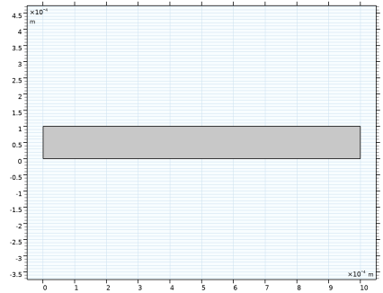
1
|
|
2
|
|
3
|
Click Add.
|
|
4
|
In the Select Physics tree, select Fluid Flow > Porous Media and Subsurface Flow > Free and Porous Media Flow, Brinkman (fp).
|
|
5
|
Click Add.
|
|
6
|
|
7
|
In the Velocity field components table, enter the following settings:
|
|
8
|
|
9
|
In the Select Physics tree, select Fluid Flow > Porous Media and Subsurface Flow > Free and Porous Media Flow, Brinkman (fp).
|
|
10
|
Click Add.
|
|
11
|
|
12
|
In the Velocity field components table, enter the following settings:
|
|
13
|
|
14
|
Click
|
|
15
|
In the Select Study tree, select Preset Studies for Selected Physics Interfaces > Hydrogen Fuel Cell > Stationary with Initialization.
|
|
16
|
Click
|
|
1
|
|
2
|
|
3
|
Click
|
|
4
|
Browse to the model’s Application Libraries folder and double-click the file sofc_unit_cell_parameters.txt.
|
|
1
|
|
2
|
|
3
|
|
4
|
Click
|
|
1
|
|
2
|
|
3
|
|
4
|
|
5
|
|
6
|
|
1
|
|
2
|
|
3
|
|
4
|
|
5
|
|
6
|
Click
|
|
1
|
|
2
|
|
3
|
|
4
|
|
5
|
|
6
|
Click
|
|
1
|
|
2
|
|
3
|
|
4
|
|
5
|
|
6
|
|
7
|
Click
|
|
1
|
|
2
|
|
3
|
|
4
|
|
5
|
|
6
|
|
7
|
|
8
|
|
1
|
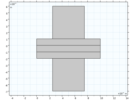
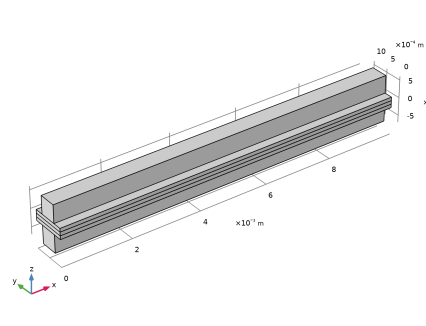
In the Model Builder window, under Component 1 (comp1) > Geometry 1 right-click Work Plane 1 (wp1) and choose Extrude.
|
|
2
|
|
4
|
Click
|
|
5
|
|
1
|
|
2
|
|
1
|
|
2
|
|
1
|
|
2
|
|
1
|
|
2
|
|
1
|
|
2
|
|
1
|
|
2
|
|
3
|
|
4
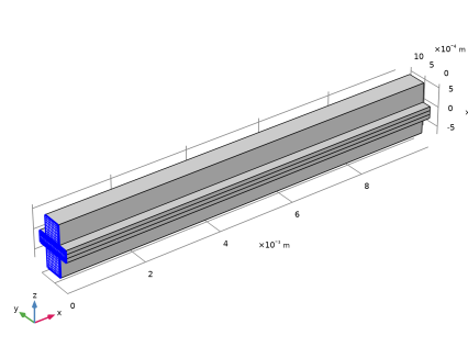
|
In the Add dialog, in the Selections to add list, choose Anode Flow Channel and Anode Gas Diffusion Electrode.
|
|
5
|
Click OK.
|
|
1
|
|
2
|
|
3
|
|
4
|
In the Add dialog, in the Selections to add list, choose Cathode Gas Diffusion Electrode and Cathode Flow Channel.
|
|
5
|
Click OK.
|
|
1
|
|
2
|
Go to the Add Material window.
|
|
3
|
In the tree, select Fuel Cell and Electrolyzer > Solid Oxides > Yttria-Stabilized Zirconia, 8YSZ, (ZrO2)0.92-(Y2O3)0.08.
|
|
4
|
Right-click and choose Add to Component 1 (comp1).
|
|
5
|
|
1
|
|
2
|
|
3
|
|
1
|
|
2
|
|
3
|
|
1
|
|
2
|
|
3
|
|
1
|
|
2
|
|
3
|
|
4
|
|
5
|
Locate the Effective Electrolyte Charge Transport section. From the Effective conductivity correction list, choose User defined. In the fl text field, type fl_a.
|
|
6
|
|
7
|
Select the Include pore-wall interaction checkbox.
|
|
8
|
|
1
|
|
2
|
In the Settings window for H2 Gas Diffusion Electrode Reaction, locate the Electrode Kinetics section.
|
|
3
|
|
4
|
|
5
|
|
6
|
|
7
|
|
8
|
|
9
|
|
1
|
|
2
|
|
3
|
|
4
|
|
5
|
Locate the Effective Electrolyte Charge Transport section. From the Effective conductivity correction list, choose User defined. In the fl text field, type fl_c.
|
|
6
|
|
7
|
Select the Include pore-wall interaction checkbox.
|
|
8
|
|
1
|
|
2
|
In the Settings window for O2 Gas Diffusion Electrode Reaction, locate the Electrode Kinetics section.
|
|
3
|
|
4
|
|
5
|
|
6
|
|
7
|
|
8
|
|
1
|
|
1
|
|
3
|
|
4
|
|
1
|
In the Model Builder window, expand the Component 1 (comp1) > Hydrogen Fuel Cell (fc) > H2 Gas Phase 1 node, then click Initial Values 1.
|
|
2
|
|
3
|
|
1
|
|
3
|
|
4
|
Click
|
|
5
|
|
6
|
Click OK.
|
|
7
|
|
8
|
From the list, choose Mass flow rates.
|
|
1
|
|
3
|
|
4
|
Click
|
|
5
|
|
6
|
Click OK.
|
|
1
|
In the Model Builder window, expand the Component 1 (comp1) > Hydrogen Fuel Cell (fc) > O2 Gas Phase 1 node, then click Initial Values 1.
|
|
2
|
|
3
|
|
1
|
|
3
|
|
4
|
Click
|
|
5
|
|
6
|
Click OK.
|
|
7
|
|
8
|
From the list, choose Mass flow rates.
|
|
9
|
|
10
|
|
1
|
|
3
|
|
4
|
Click
|
|
5
|
|
6
|
Click OK.
|
|
1
|
In the Model Builder window, under Component 1 (comp1) click Free and Porous Media Flow, Brinkman (fp).
|
|
2
|
In the Settings window for Free and Porous Media Flow, Brinkman, type Free and Porous Media Flow - Cathode in the Label text field.
|
|
3
|
|
4
|
In the Model Builder window, under Component 1 (comp1) click Free and Porous Media Flow - Cathode (fp).
|
|
5
|
Locate the Physical Model section. From the Compressibility list, choose Compressible flow (Ma<0.3).
|
|
6
|
|
1
|
|
2
|
|
3
|
|
1
|
|
2
|
|
3
|
|
4
|
|
1
|
|
2
|
|
3
|
|
4
|
|
5
|
|
6
|
|
1
|
|
2
|
|
3
|
|
4
|
|
1
|
In the Model Builder window, under Component 1 (comp1) click Free and Porous Media Flow, Brinkman 2 (fp2).
|
|
2
|
In the Settings window for Free and Porous Media Flow, Brinkman, type Free and Porous Media Flow - Anode in the Label text field.
|
|
3
|
|
4
|
In the Model Builder window, under Component 1 (comp1) click Free and Porous Media Flow - Anode (fp2).
|
|
5
|
Locate the Physical Model section. From the Compressibility list, choose Compressible flow (Ma<0.3).
|
|
6
|
|
1
|
|
2
|
|
3
|
|
1
|
|
2
|
|
3
|
|
4
|
|
1
|
|
2
|
|
3
|
|
4
|
|
5
|
|
1
|
|
2
|
|
3
|
|
4
|
|
1
|
In the Physics toolbar, click
|
|
2
|
|
3
|
|
1
|
|
2
|
|
3
|
|
4
|
|
1
|
|
1
|
|
2
|
|
3
|
Click the Custom button.
|
|
4
|
Locate the Element Size Parameters section.
|
|
5
|
|
6
|
Click
|
|
1
|
|
1
|
|
3
|
|
4
|
|
5
|
|
6
|
|
7
|
Select the Symmetric distribution checkbox.
|
|
1
|
|
3
|
|
4
|
|
5
|
|
6
|
|
1
|
|
2
|
|
3
|
Click
|
|
5
|
|
1
|
|
3
|
|
4
|
|
1
|
|
2
|
|
3
|
Click the Custom button.
|
|
4
|
Locate the Element Size Parameters section.
|
|
5
|
|
6
|
Click
|
|
7
|
|
1
|
|
2
|
|
3
|
|
4
|
|
5
|
Click Replace Expression in the upper-right corner of the Expression section. From the menu, choose Component 1 (comp1) > Hydrogen Fuel Cell > Electrode kinetics > fc.ivtot - Electrode reaction source - A/m³.
|
|
6
|
|
7
|
|
1
|
|
2
|
In the Settings window for Current Distribution Initialization, locate the Physics and Variables Selection section.
|
|
3
|
In the Solve for column of the table, under Component 1 (comp1) > Multiphysics, clear the checkboxes for Reacting Flow, H2 Gas Phase 1 (rfh1) and Reacting Flow, O2 Gas Phase 1 (rfo1).
|
|
1
|
|
2
|
|
3
|
In the Solve for column of the table, under Component 1 (comp1), clear the checkboxes for Hydrogen Fuel Cell (fc) and Free and Porous Media Flow - Anode (fp2).
|
|
4
|
In the Solve for column of the table, under Component 1 (comp1) > Multiphysics, clear the checkboxes for Reacting Flow, H2 Gas Phase 1 (rfh1) and Reacting Flow, O2 Gas Phase 1 (rfo1).
|
|
1
|
|
2
|
|
3
|
In the Solve for column of the table, under Component 1 (comp1), clear the checkboxes for Hydrogen Fuel Cell (fc) and Free and Porous Media Flow - Cathode (fp).
|
|
4
|
In the Solve for column of the table, under Component 1 (comp1) > Multiphysics, clear the checkboxes for Reacting Flow, H2 Gas Phase 1 (rfh1) and Reacting Flow, O2 Gas Phase 1 (rfo1).
|
|
1
|
|
2
|
|
3
|
Select the Auxiliary sweep checkbox.
|
|
4
|
Click
|
|
1
|
|
2
|
|
3
|
In the Model Builder window, expand the Study 1 > Solver Configurations > Solution 1 (sol1) > Stationary Solver 4 node.
|
|
4
|
Right-click Study 1 > Solver Configurations > Solution 1 (sol1) > Stationary Solver 4 and choose Fully Coupled.
|
|
5
|
|
1
|
|
2
|
|
3
|
|
4
|
Locate the Plot Settings section.
|
|
5
|
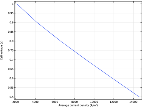
Select the x-axis label checkbox. In the associated text field, type Average current density (A/m<sup>2</sup>).
|
|
6
|
|
7
|
|
1
|
|
2
|
|
4
|
|
5
|
|
6
|
|
1
|
|
2
|
|
3
|
|
4
|
Locate the Plot Settings section.
|
|
5
|
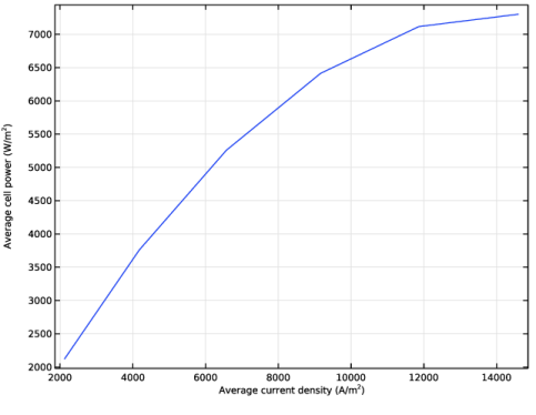
Select the x-axis label checkbox. In the associated text field, type Average current density (A/m<sup>2</sup>).
|
|
6
|
Select the y-axis label checkbox. In the associated text field, type Average cell power (W/m<sup>2</sup>).
|
|
7
|
|
1
|
|
2
|
|
4
|
|
5
|
|
6
|
|
1
|
|
2
|
|
3
|
|
1
|
|
2
|
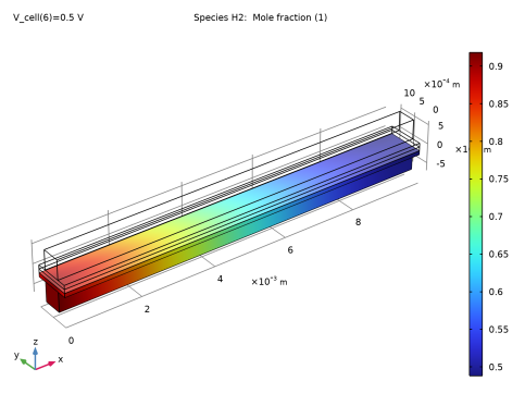
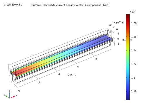
In the Settings window for Surface, click Replace Expression in the upper-right corner of the Expression section. From the menu, choose Component 1 (comp1) > Hydrogen Fuel Cell > Electrolyte current density vector - A/m² > fc.Ilz - Electrolyte current density vector, z-component.
|
|
3
|
|
4
|
|
1
|
In the Model Builder window, under Component 1 (comp1) right-click Definitions and choose Variables.
|
|
2
|
|
3
|
Click
|
|
4
|
Browse to the model’s Application Libraries folder and double-click the file sofc_unit_cell_variables.txt.
|
|
1
|
|
2
|
|
3
|
|
1
|
|
2
|
|
3
|
|
1
|
|
2
|
|
3
|
Locate the Source Selection section. From the Selection list, choose Cathode Gas Diffusion Electrode.
|
|
1
|
|
2
|
|
3
|
|
1
|
|
1
|
|
2
|
|
1
|
|
2
|
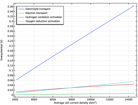
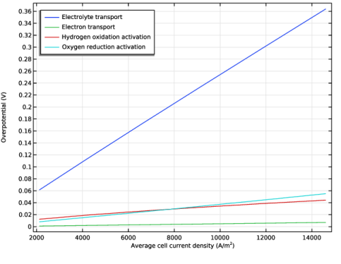
In the Settings window for Global, click Add Expression in the upper-right corner of the y-Axis Data section. From the menu, choose Component 1 (comp1) > Definitions > Variables > eta_phil - Cell-averaged electrolyte transport overpotential - V.
|
|
3
|
Click Add Expression in the upper-right corner of the y-Axis Data section. From the menu, choose Component 1 (comp1) > Definitions > Variables > eta_phis - Cell-averaged electron transport overpotential - V.
|
|
4
|
Click Add Expression in the upper-right corner of the y-Axis Data section. From the menu, choose Component 1 (comp1) > Definitions > Variables > eta_act_h2 - Cell-averaged hydrogen oxidation activation overpotential - V.
|
|
5
|
Click Add Expression in the upper-right corner of the y-Axis Data section. From the menu, choose Component 1 (comp1) > Definitions > Variables > eta_act_o2 - Cell-averaged oxygen reduction activation overpotential - V.
|
|
6
|
Click Replace Expression in the upper-right corner of the x-Axis Data section. From the menu, choose Component 1 (comp1) > Definitions > I_cell - Cell Current Density Probe - A/m².
|
|
7
|
|
8
|
|
1
|
|
2
|
|
3
|
Select the x-axis label checkbox. In the associated text field, type Average cell current density (A/m<sup>2</sup>).
|
|
4
|
|
5
|
|
6
|
|
7
|