|
|
|


|
1
|
|
2
|
|
3
|
Click Add.
|
|
4
|
Click
|
|
5
|
|
6
|
Click
|
|
1
|
|
2
|
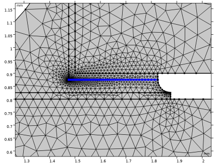
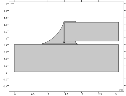
Browse to the model’s Application Libraries folder and double-click the file surface_mount_resistor_geom_sequence.mph.
|
|
3
|
|
4
|
|
5
|
|
1
|
|
2
|
|
3
|
|
4
|
Click
|
|
5
|
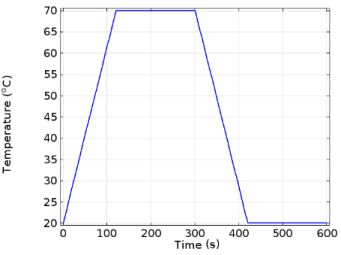
Browse to the model’s Application Libraries folder and double-click the file surface_mount_resistor_thermal_load_cycle.txt.
|
|
6
|
Click
|
|
7
|
|
8
|
|
9
|
In the Function table, enter the following settings:
|
|
1
|
|
2
|
|
3
|
|
4
|
|
1
|
|
2
|
In the Show More Options dialog, in the tree, select the checkbox for the node Physics > Advanced Physics Options.
|
|
3
|
Click OK.
|
|
4
|
In the Model Builder window, under Component 1 (comp1) > Solid Mechanics (solid) click Linear Elastic Material 1.
|
|
5
|
|
6
|
Select the Calculate dissipated energy checkbox.
|
|
1
|
|
2
|
|
3
|
|
1
|
|
2
|
|
3
|
|
4
|
Locate the Model Input section. From the T list, choose User defined. In the associated text field, type thermLC(t).
|
|
5
|
|
6
|
|
7
|
|
8
|
|
9
|
|
1
|
|
1
|
|
1
|
In the Model Builder window, under Component 1 (comp1) right-click Materials and choose Blank Material.
|
|
2
|
|
3
|
|
4
|
Locate the Material Contents section. In the table, enter the following settings:
|
|
1
|
|
2
|
|
3
|
|
4
|
Locate the Material Contents section. In the table, enter the following settings:
|
|
1
|
|
2
|
|
3
|
|
4
|
Locate the Material Contents section. In the table, enter the following settings:
|
|
1
|
|
2
|
|
3
|
|
4
|
Locate the Material Contents section. In the table, enter the following settings:
|
|
1
|
|
2
|
|
3
|
|
4
|
Locate the Material Contents section. In the table, enter the following settings:
|
|
1
|
|
2
|
|
3
|
|
1
|
|
3
|
|
4
|
|
5
|
|
6
|
|
7
|
|
1
|
|
2
|
|
3
|
|
4
|
|
5
|
|
6
|
|
7
|
|
1
|
|
2
|
|
3
|
|
4
|
|
5
|
In the Model Builder window, expand the Time History > Solver Configurations > Solution 1 (sol1) > Time-Dependent Solver 1 node.
|
|
6
|
|
1
|
|
2
|
|
3
|
Click
|
|
4
|
|
5
|
Click OK.
|
|
6
|
|
8
|
Click
|
|
1
|
|
2
|
|
3
|
|
4
|
|
1
|
|
2
|
Go to the Result Templates window.
|
|
3
|
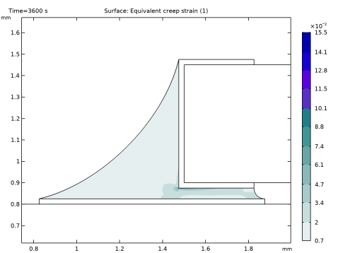
In the tree, select Time History/Solution 1 (sol1) > Solid Mechanics > Equivalent Creep Strain (solid).
|
|
4
|
Click the Add Result Template button in the window toolbar.
|
|
5
|
|
1
|
|
2
|
|
3
|
|
1
|
|
2
|
|
3
|
|
4
|
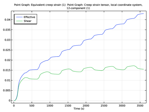
Click Replace Expression in the upper-right corner of the y-Axis Data section. From the menu, choose Component 1 (comp1) > Solid Mechanics > Strain > solid.eceGp - Equivalent creep strain - 1.
|
|
5
|
|
6
|
|
1
|
|
2
|
In the Settings window for Point Graph, click Replace Expression in the upper-right corner of the y-Axis Data section. From the menu, choose Component 1 (comp1) > Solid Mechanics > Strain > Creep strain tensor, local coordinate system > solid.eclGp12 - Creep strain tensor, local coordinate system, 12-component.
|
|
3
|
Locate the Legends section. In the table, enter the following settings:
|
|
1
|
|
2
|
|
3
|
|
4
|
|
1
|
|
2
|
|
1
|
|
2
|
|
3
|
|
4
|
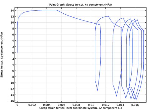
Click Replace Expression in the upper-right corner of the y-Axis Data section. From the menu, choose Component 1 (comp1) > Solid Mechanics > Stress > Stress tensor (spatial frame) - N/m² > solid.sGpxy - Stress tensor, xy-component.
|
|
5
|
|
6
|
Click Replace Expression in the upper-right corner of the x-Axis Data section. From the menu, choose Component 1 (comp1) > Solid Mechanics > Strain > Creep strain tensor, local coordinate system > solid.eclGp12 - Creep strain tensor, local coordinate system, 12-component.
|
|
7
|
|
1
|
|
2
|
Go to the Add Physics window.
|
|
3
|
|
4
|
Find the Physics interfaces in study subsection. In the table, clear the Solve checkbox for Time History.
|
|
5
|
Click the Add to Component 1 button in the window toolbar.
|
|
1
|
|
2
|
|
3
|
|
4
|
|
5
|
|
6
|
|
1
|
Go to the Add Physics window.
|
|
2
|
|
3
|
Find the Physics interfaces in study subsection. In the table, clear the Solve checkbox for Time History.
|
|
4
|
Click the Add to Component 1 button in the window toolbar.
|
|
5
|
|
1
|
|
2
|
|
3
|
|
4
|
|
5
|
Locate the Fatigue Model Selection section. From the Energy type list, choose Creep dissipation density.
|
|
1
|
In the Model Builder window, expand the Component 1 (comp1) > Materials > Solder (mat3) node, then click Solder (mat3).
|
|
2
|
|
3
|
|
4
|
Click
|
|
5
|
In the Material properties tree, select Solid Mechanics > Fatigue Behavior > Strain-Based > Coffin–Manson.
|
|
6
|
Click
|
|
7
|
In the Model Builder window, under Component 1 (comp1) > Materials > Solder (mat3) click Morrow (fatigueEnergyMorrow).
|
|
8
|
|
10
|
In the Model Builder window, under Component 1 (comp1) > Materials > Solder (mat3) click Coffin–Manson (fatigueStrainCoffinManson).
|
|
11
|
|
1
|
|
2
|
Go to the Add Study window.
|
|
3
|
Find the Physics interfaces in study subsection. In the table, clear the Solve checkbox for Solid Mechanics (solid).
|
|
4
|
Find the Studies subsection. In the Select Study tree, select Preset Studies for Selected Physics Interfaces > Fatigue.
|
|
5
|
Click the Add Study button in the window toolbar.
|
|
6
|
|
1
|
|
2
|
|
3
|
Find the Values of variables not solved for subsection. From the Settings list, choose User controlled.
|
|
4
|
|
5
|
|
6
|
|
7
|
From the Time (s) selection list, select time steps from 3000 s to 3600 s.
|
|
8
|
|
1
|
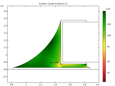
In the Settings window for 2D Plot Group, type Cycles to Failure, Coffin-Manson in the Label text field.
|
|
2
|
|
1
|
In the Model Builder window, expand the Results > Cycles to Failure, Coffin-Manson > Surface 1 node, then click Marker 1.
|
|
2
|
|
3
|
|
1
|
|
2
|
|
3
|
|
1
|
In the Model Builder window, expand the Results > Cycles to Failure, Morrow > Surface 1 node, then click Marker 1.
|
|
2
|
|
3
|
|
1
|
|
2
|
|
3
|
|
1
|
|
2
|
|
3
|
|
4
|
|
5
|
Locate the Selections of Resulting Entities section. Select the Resulting objects selection checkbox.
|
|
1
|
|
2
|
|
3
|
|
4
|
|
5
|
|
6
|
|
7
|
Locate the Selections of Resulting Entities section. Select the Resulting objects selection checkbox.
|
|
1
|
|
2
|
|
3
|
|
4
|
|
5
|
|
6
|
|
7
|
Locate the Selections of Resulting Entities section. Select the Resulting objects selection checkbox.
|
|
1
|
|
2
|
|
3
|
|
4
|
|
5
|
|
6
|
|
7
|
Locate the Selections of Resulting Entities section. Find the Cumulative selection subsection. Click New.
|
|
8
|
|
9
|
Click OK.
|
|
10
|
|
1
|
|
2
|
|
3
|
|
4
|
|
5
|
|
6
|
|
7
|
|
8
|
|
9
|
Click
|
|
1
|
|
2
|
|
3
|
|
4
|
Locate the Coordinates section. In the table, enter the following settings:
|
|
5
|
Click
|
|
1
|
|
2
|
|
3
|
|
4
|
|
5
|
|
6
|
|
7
|
|
8
|
Click
|
|
1
|
|
2
|
On the object ca1, select Point 2 only.
|
|
3
|
|
4
|
|
5
|
On the object qb1, select Point 1 only.
|
|
6
|
Click
|
|
1
|
|
2
|
|
3
|
|
4
|
|
5
|
|
6
|
Click OK.
|
|
7
|
|
1
|
|
2
|
|
3
|
|
4
|
|
5
|
Locate the Selections of Resulting Entities section. Select the Resulting objects selection checkbox.
|
|
6
|
Click
|
|
1
|
|
2
|
|
3
|
|
1
|
Click
|
|
2
|