|
|
|

|
1
|
|
2
|
In the Select Physics tree, select Electrochemistry > Electrodeposition, Deformed Geometry > Electrodeposition, Tertiary with Supporting Electrolyte.
|
|
3
|
Click Add.
|
|
4
|
|
5
|
In the Concentrations (mol/m³) table, enter the following settings:
|
|
6
|
Click
|
|
7
|
In the Select Study tree, select Preset Studies for Selected Physics Interfaces > Time Dependent with Initialization.
|
|
8
|
Click
|
|
1
|
|
2
|
|
3
|
Click
|
|
4
|
Browse to the model’s Application Libraries folder and double-click the file inductor_coil_parameters.txt.
|
|
1
|
|
2
|
|
3
|
|
4
|
|
5
|
Locate the Units section. In the table, enter the following settings:
|
|
6
|
|
1
|
|
2
|
|
3
|
|
4
|
|
5
|
Locate the Units section. In the table, enter the following settings:
|
|
6
|
|
1
|
|
2
|
|
1
|
|
2
|
|
3
|
|
4
|
|
5
|
|
6
|
Click
|
|
1
|
|
2
|
|
3
|
|
4
|
|
5
|
|
6
|
Click
|
|
1
|
|
2
|
|
3
|
|
4
|
|
5
|
|
6
|
Click
|
|
1
|
|
2
|
|
3
|
|
4
|
|
5
|
|
6
|
Click
|
|
1
|
|
2
|
|
3
|
|
4
|
|
5
|
|
6
|
Click
|
|
1
|
|
2
|
|
3
|
|
4
|
|
5
|
|
6
|
|
7
|
Click
|
|
1
|
|
2
|
|
3
|
|
4
|
|
5
|
|
6
|
Click
|
|
1
|
|
2
|
Click in the Graphics window and then press Ctrl+A to select all objects.
|
|
3
|
|
1
|
In the Model Builder window, under Component 1 (comp1) > Geometry 1 right-click Work Plane 1 (wp1) and choose Extrude.
|
|
2
|
|
4
|
Click
|
|
1
|
|
2
|
|
3
|
|
4
|
|
5
|
|
6
|
|
7
|
|
8
|
|
9
|
Click
|
|
1
|
|
1
|
|
3
|
|
1
|
|
2
|
|
3
|
|
4
|
|
5
|
Click OK.
|
|
6
|
|
1
|
|
2
|
|
3
|
Select the All domains checkbox.
|
|
4
|
|
5
|
|
1
|
|
2
|
|
3
|
|
5
|
|
1
|
|
2
|
|
3
|
|
4
|
Click
|
|
5
|
|
6
|
Click OK.
|
|
7
|
|
1
|
|
2
|
|
3
|
|
4
|
|
5
|
Click OK.
|
|
6
|
|
1
|
|
2
|
|
3
|
|
4
|
|
5
|
|
6
|
Click OK.
|
|
7
|
|
8
|
|
9
|
|
10
|
Click OK.
|
|
11
|
|
1
|
In the Model Builder window, under Component 1 (comp1) click Tertiary Current Distribution, Nernst-Planck (tcd).
|
|
2
|
In the Settings window for Tertiary Current Distribution, Nernst-Planck, locate the Electrolyte Charge Conservation section.
|
|
3
|
|
1
|
In the Model Builder window, under Component 1 (comp1) > Tertiary Current Distribution, Nernst-Planck (tcd) click Electrolyte 1.
|
|
2
|
|
3
|
|
1
|
|
2
|
|
3
|
|
1
|
|
2
|
|
3
|
|
4
|
|
5
|
Locate the Electrode Phase Potential Condition section. From the Electrode phase potential condition list, choose Average current density.
|
|
6
|
|
1
|
|
2
|
|
3
|
|
4
|
|
5
|
In the Stoichiometric coefficients for dissolving-depositing species: table, enter the following settings:
|
|
6
|
|
7
|
|
8
|
|
1
|
|
2
|
|
3
|
|
4
|
|
5
|
|
6
|
|
7
|
In the Settings window for Tertiary Current Distribution, Nernst-Planck, click to expand the Discretization section.
|
|
8
|
|
9
|
|
1
|
|
2
|
|
3
|
|
1
|
In the Model Builder window, under Component 1 (comp1) > Multiphysics click Nondeforming Boundary 1 (ndbdg1).
|
|
2
|
|
3
|
|
1
|
|
2
|
|
3
|
|
4
|
Locate the Nondeforming Boundary section. From the Boundary condition list, choose Zero normal displacement.
|
|
5
|
Select the Allow deformation along specified line only checkbox.
|
|
6
|
|
1
|
|
2
|
|
3
|
From the list, choose User-controlled mesh.
|
|
4
|
|
1
|
|
3
|
|
4
|
Select the Adjust edge mesh checkbox.
|
|
1
|
|
2
|
|
3
|
Click the Custom button.
|
|
4
|
Locate the Element Size Parameters section.
|
|
5
|
|
6
|
|
1
|
|
1
|
|
2
|
|
3
|
Click the Custom button.
|
|
4
|
Locate the Element Size Parameters section.
|
|
5
|
|
6
|
|
1
|
|
2
|
|
3
|
|
4
|
|
1
|
|
2
|
|
1
|
|
2
|
|
1
|
|
2
|
|
3
|
Clear the Generate default plots checkbox.
|
|
1
|
|
2
|
|
3
|
|
4
|
|
1
|
|
2
|
|
3
|
|
4
|
|
5
|
Clear the Plot dataset edges checkbox.
|
|
1
|
|
2
|
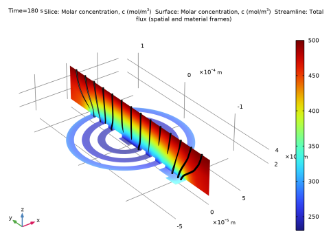
In the Settings window for Slice, click Replace Expression in the upper-right corner of the Expression section. From the menu, choose Component 1 (comp1) > Tertiary Current Distribution, Nernst-Planck > Species c > c - Molar concentration, c - mol/m³.
|
|
3
|
|
4
|
|
1
|
|
2
|
|
3
|
|
4
|
|
1
|
|
2
|
|
3
|
|
1
|
|
2
|
In the Settings window for Streamline, click Replace Expression in the upper-right corner of the Expression section. From the menu, choose Component 1 (comp1) > Tertiary Current Distribution, Nernst-Planck > Species c > Fluxes > tcd.tflux_cx,...,tcd.tflux_cz - Total flux (spatial and material frames).
|
|
3
|
Locate the Streamline Positioning section. From the Positioning list, choose Starting-point controlled.
|
|
4
|
|
5
|
|
6
|
|
7
|
|
8
|
Locate the Coloring and Style section. Find the Line style subsection. From the Type list, choose Tube.
|
|
9
|
|
10
|
|
11
|
|
1
|
|
2
|
|
3
|
|
4
|
|
5
|
|
1
|
|
2
|
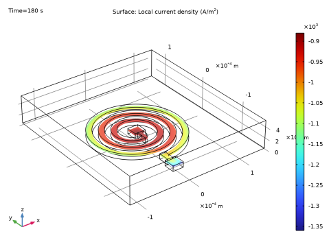
In the Settings window for Surface, click Replace Expression in the upper-right corner of the Expression section. From the menu, choose Component 1 (comp1) > Tertiary Current Distribution, Nernst-Planck > Electrode kinetics > tcd.iloc_er1 - Local current density - A/m².
|
|
3
|
|
4
|
|
1
|
|
2
|
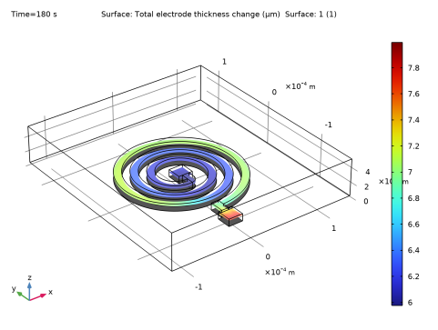
In the Settings window for Surface, click Replace Expression in the upper-right corner of the Expression section. From the menu, choose Component 1 (comp1) > Tertiary Current Distribution, Nernst-Planck > Dissolving-depositing species > tcd.sbtot - Total electrode thickness change - m.
|
|
3
|
|
1
|
|
2
|
|
3
|
|
4
|
|
5
|
|
6
|
|
7
|
|
1
|
|
2
|
|
3
|
|
4
|
|
5
|