
|
|
|
|
{230,15} GPa
|
|
|
G12
|
27 GPa
|
|
•
|
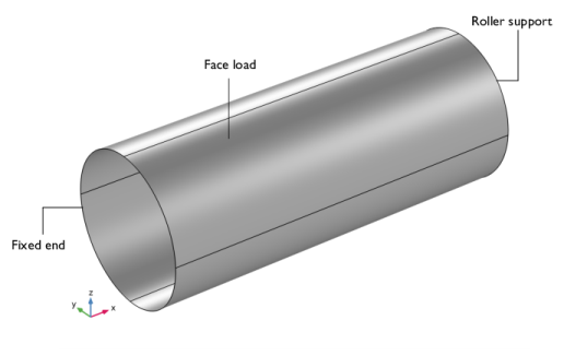
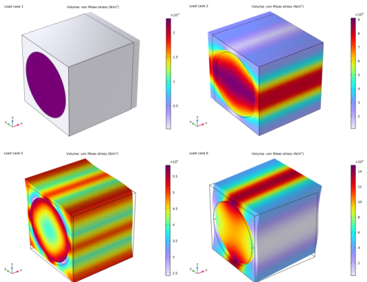
A load of 1 kN is applied to a quarter of the cylinder outer surface.
|
|
•
|
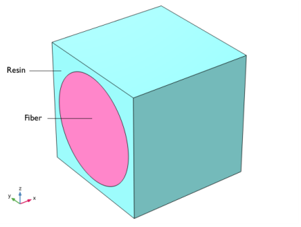
The micromechanics analysis of a single fiber in a resin can be performed using the Cell Periodicity node available in the Solid Mechanics interface. Using this functionality, the elasticity matrix of the homogenized material can be computed for the given fiber and resin properties, and the fiber volume fraction.
|
|
•
|
The Cell Periodicity node has three action buttons on the tool bar of section called Periodicity Type: Create Load Groups and Study, Create Material by Reference, and Create Material by Value. The action button Create Load Groups and Study generates load groups and a stationary study with load cases. The action button Create Material by Reference generates a Global Material with an elasticity matrix corresponding to that of the homogenized material in terms of variables. The action button Create Material by Value generates a Global Material with an elasticity matrix corresponding to that of the homogenized material in terms of numbers after the study computed. The action buttons are active depending on the choices in the Periodicity Type and Calculate Average Properties lists.
|
|
•
|
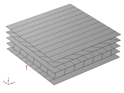
Modeling a composite laminated shell requires a surface geometry (2D), in general called a base surface, and a Layered Material node which adds an extra dimension (1D) to the base surface geometry in the surface normal direction. Using the Layered Material functionality, you can model several layers of different thickness, material properties, and fiber orientations. You can optionally specify the interface materials between the layers and the control mesh elements in each layer.
|
|
•
|
The Layered Material Link and Layered Material Stack have an option to transform the given Layered Material into a symmetric or antisymmetric laminate. A repeated laminate can also be constructed using a transform option.
|
|
•
|
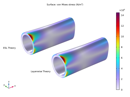
You can either use the Layerwise (LW) theory based Layered Shell interface or the Equivalent Single Layer (ESL) theory based Linear Elastic Material, Layered node in Shell interface.
|
|
•
|
The built-in Composites material library contains data for fiber and matrix constituents as well as for unidirectional and bidirectional laminae.
|
|
•
|
To analyze the results in a composite shell, you can either create a slice plot using the Layered Material Slice plot for in-plane variation of a quantity, or you can create a Through Thickness plot for out-of-plane variation of a quantity at a point. To visualize the results as a 3D solid object, you can use the Layered Material dataset which creates a virtual 3D solid object combining the surface geometry (2D) and the extra dimension (1D).
|
|
1
|
|
2
|
|
3
|
Click Add.
|
|
4
|
Click
|
|
1
|
|
2
|
|
3
|
Click
|
|
4
|
Browse to the model’s Application Libraries folder and double-click the file composite_cylinder_micromechanics_and_stress_analysis_parameters.txt.
|
|
5
|
In the Model Builder window, right-click Global Definitions and choose Geometry Parts > Part Libraries.
|
|
1
|
In the Part Libraries window, select COMSOL Multiphysics > Unit Cells and RVEs > Fiber Composites > unidirectional_fiber_square_packing in the tree.
|
|
2
|
Click
|
|
3
|
In the Select Part Variant dialog, select Specify fiber volume fraction in the Select part variant list.
|
|
4
|
Click OK.
|
|
1
|
In the Geometry toolbar, click
|
|
2
|
|
1
|
|
2
|
|
1
|
In the Model Builder window, under Component 1 (comp1) > Solid Mechanics (solid) click Linear Elastic Material 1.
|
|
2
|
|
3
|
|
1
|
|
2
|
|
3
|
|
4
|
|
5
|
Select the Compute elasticity matrix, standard notation checkbox.
|
|
1
|
|
2
|
|
3
|
Click
|
|
1
|
|
2
|
|
3
|
Click
|
|
1
|
|
2
|
|
3
|
Click
|
|
1
|
|
2
|
In the Settings window for Cell Periodicity, click Automated Model Setup in the upper-right corner of the Periodicity Settings section. From the menu, choose Create Load Groups and Study to generate load groups and a study node.
|
|
1
|
In the Model Builder window, under Component 1 (comp1) right-click Materials and choose More Materials > Material Link.
|
|
2
|
|
3
|
Locate the Geometric Entity Selection section. From the Selection list, choose Matrix (Unidirectional Fiber Composite, Square Packing 1).
|
|
4
|
|
1
|
Go to the Add Material to Material Link 1: Matrix (matlnk1) window.
|
|
2
|
|
3
|
Click OK.
|
|
1
|
|
2
|
|
3
|
Locate the Geometric Entity Selection section. From the Selection list, choose Fiber (Unidirectional Fiber Composite, Square Packing 1).
|
|
4
|
|
1
|
Go to the Add Material to Material Link 2: Fiber (matlnk2) window.
|
|
2
|
|
3
|
Click OK.
|
|
1
|
|
2
|
|
3
|
Click the Predefined button.
|
|
1
|
|
2
|
|
3
|
|
4
|
Locate the Second Entity Group section. From the Selection list, choose Pair 1, Destination (Unidirectional Fiber Composite, Square Packing 1).
|
|
1
|
|
2
|
|
3
|
|
4
|
Click
|
|
1
|
|
2
|
|
1
|
|
2
|
|
1
|
In the Model Builder window, under Component 1 (comp1) > Solid Mechanics (solid) click Cell Periodicity 1.
|
|
2
|
In the Settings window for Cell Periodicity, click Automated Model Setup in the upper-right corner of the Periodicity Settings section. From the menu, choose Create Material by Value to generate a global material node with computed density and elastic properties.
|
|
1
|
|
2
|
|
3
|
|
4
|
|
5
|
|
6
|
|
7
|
Click
|
|
1
|
In the Model Builder window, expand the Component 2 (comp2) > Definitions node, then click Boundary System 2 (sys2).
|
|
2
|
|
3
|
|
1
|
|
2
|
Go to the Add Physics window.
|
|
3
|
|
4
|
Find the Physics interfaces in study subsection. In the table, clear the Solve checkbox for Cell Periodicity Study.
|
|
5
|
Click the Add to Component 2 button in the window toolbar.
|
|
6
|
|
1
|
In the Model Builder window, under Global Definitions right-click Materials and choose Layered Material.
|
|
2
|
In the Settings window for Layered Material, type Layered Material: [0/45/90/-45/0] in the Label text field.
|
|
3
|
Locate the Layer Definition section. In the table, enter the following settings:
|
|
4
|
Click Add two times.
|
|
1
|
In the Model Builder window, under Component 2 (comp2) right-click Materials and choose Layers > Layered Material Link.
|
|
2
|
|
3
|
|
4
|
Select the Merge middle layers checkbox.
|
|
5
|
Click to expand the Preview Plot Settings section. In the Thickness-to-width ratio text field, type 0.4.
|
|
6
|
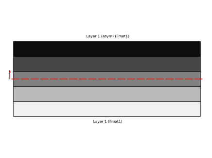
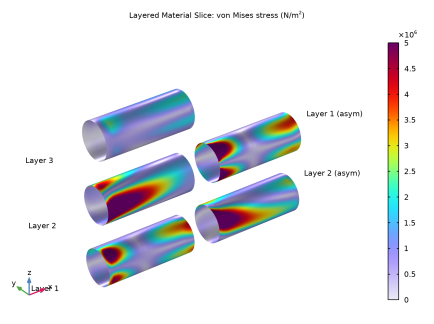
Locate the Layered Material Settings section. Click Layer Cross-Section Preview in the upper-right corner of the section to enable the through-thickness view of the laminated material as in Figure 3.
|
|
7
|
|
1
|
In the Model Builder window, under Component 2 (comp2) > Layered Shell (lshell) click Linear Elastic Material 1.
|
|
2
|
|
3
|
|
1
|
|
1
|
|
1
|
|
3
|
|
4
|
|
5
|
|
1
|
|
2
|
|
3
|
|
1
|
|
2
|
|
3
|
|
4
|
|
5
|
Click
|
|
1
|
|
2
|
Go to the Add Study window.
|
|
3
|
|
4
|
Find the Physics interfaces in study subsection. In the table, clear the Solve checkbox for Solid Mechanics (solid).
|
|
5
|
Click the Add Study button in the window toolbar.
|
|
6
|
|
1
|
In the Settings window for Study, type Study 1: Stationary (Layerwise Theory) in the Label text field.
|
|
2
|
|
1
|
|
2
|
|
3
|
|
1
|
|
2
|
|
3
|
|
4
|
|
5
|
|
6
|
|
7
|
|
1
|
|
2
|
|
3
|
|
4
|
|
1
|
|
2
|
Go to the Result Templates window.
|
|
3
|
In the tree, select Study 1: Stationary (Layerwise Theory)/Solution 1 (3) (sol1) > Layered Shell > Stress, Slice (lshell).
|
|
4
|
Click the Add Result Template button in the window toolbar.
|
|
1
|
|
2
|
|
1
|
In the Model Builder window, expand the Stress, Slice (mises) node, then click Layered Material Slice 1.
|
|
2
|
|
3
|
|
4
|
|
5
|
|
6
|
|
7
|
|
8
|
Select the Show descriptions checkbox.
|
|
9
|
|
10
|
|
11
|
|
12
|
|
13
|
|
1
|
|
2
|
|
1
|
|
2
|
|
1
|
Go to the Result Templates window.
|
|
2
|
In the tree, select Study 1: Stationary (Layerwise Theory)/Solution 1 (3) (sol1) > Layered Shell > Stress, Through Thickness (lshell).
|
|
3
|
Click the Add Result Template button in the window toolbar.
|
|
1
|
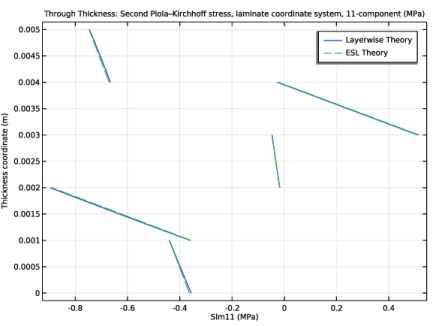
In the Settings window for 1D Plot Group, type Stress, Through Thickness (Slm11) in the Label text field.
|
|
2
|
Locate the Plot Settings section.
|
|
3
|
|
1
|
In the Model Builder window, expand the Stress, Through Thickness (Slm11) node, then click Through Thickness 1.
|
|
2
|
|
3
|
|
4
|
|
5
|
|
6
|
|
8
|
|
1
|
Go to the Result Templates window.
|
|
2
|
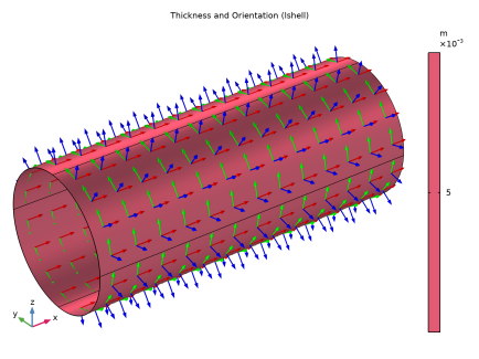
In the tree, select Study 1: Stationary (Layerwise Theory)/Solution 1 (3) (sol1) > Layered Shell > Geometry and Layup (lshell) > Thickness and Orientation (lshell).
|
|
3
|
Click the Add Result Template button in the window toolbar.
|
|
4
|
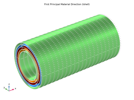
In the tree, select Study 1: Stationary (Layerwise Theory)/Solution 1 (3) (sol1) > Layered Shell > Geometry and Layup (lshell) > First Principal Material Direction (lshell).
|
|
5
|
Click the Add Result Template button in the window toolbar.
|
|
1
|
|
2
|
|
3
|
|
1
|
|
2
|
Go to the Add Study window.
|
|
3
|
|
4
|
Find the Physics interfaces in study subsection. In the table, clear the Solve checkbox for Solid Mechanics (solid).
|
|
5
|
Click the Add Study button in the window toolbar.
|
|
6
|
|
1
|
In the Model Builder window, under Study 2: Eigenfrequency (Layerwise Theory) click Step 1: Eigenfrequency.
|
|
2
|
|
3
|
|
4
|
|
1
|
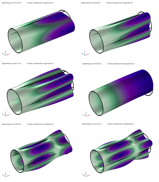
In the Settings window for 3D Plot Group, type Mode Shape (Layerwise Theory) in the Label text field.
|
|
2
|
|
3
|
|
4
|
|
1
|
|
2
|
Go to the Add Physics window.
|
|
3
|
|
4
|
Find the Physics interfaces in study subsection. In the table, clear the Solve checkboxes for Cell Periodicity Study, Study 1: Stationary (Layerwise Theory), and Study 2: Eigenfrequency (Layerwise Theory).
|
|
5
|
Click the Add to Component 2 button in the window toolbar.
|
|
6
|
|
1
|
|
2
|
In the Show More Options dialog, in the tree, select the checkbox for the node Physics > Advanced Physics Options.
|
|
3
|
Click OK.
|
|
4
|
|
5
|
Clear the Use MITC interpolation checkbox.
|
|
1
|
|
2
|
|
3
|
|
4
|
|
1
|
|
1
|
|
1
|
|
2
|
|
4
|
|
5
|
|
6
|
|
1
|
|
2
|
Go to the Add Study window.
|
|
3
|
|
4
|
Find the Physics interfaces in study subsection. In the table, clear the Solve checkboxes for Solid Mechanics (solid) and Layered Shell (lshell).
|
|
5
|
Click the Add Study button in the window toolbar.
|
|
6
|
|
1
|
|
2
|
|
3
|
|
1
|
|
2
|
|
3
|
|
4
|
|
1
|
In the Model Builder window, under Results > Datasets right-click Cut Point 3D 1 and choose Duplicate.
|
|
2
|
|
3
|
|
1
|
|
2
|
|
3
|
|
4
|
|
5
|
|
6
|
|
7
|
|
1
|
|
2
|
|
3
|
|
4
|
|
5
|
|
1
|
|
2
|
|
3
|
|
5
|
|
6
|
|
1
|
|
2
|
|
3
|
Select the Enable checkbox.
|
|
4
|
|
5
|
|
6
|
|
1
|
In the Model Builder window, under Results > Stress, Through Thickness (Slm11) right-click Through Thickness 1 and choose Duplicate.
|
|
2
|
|
3
|
|
4
|
|
5
|
|
6
|
Click to expand the Coloring and Style section. Find the Line style subsection. From the Line list, choose Dashed.
|
|
7
|
Locate the Legends section. In the table, enter the following settings:
|
|
8
|
|
1
|
|
2
|
Go to the Add Study window.
|
|
3
|
|
4
|
Find the Physics interfaces in study subsection. In the table, clear the Solve checkboxes for Solid Mechanics (solid) and Layered Shell (lshell).
|
|
5
|
Click the Add Study button in the window toolbar.
|
|
6
|
|
1
|
In the Settings window for Study, type Study 4: Eigenfrequency (ESL Theory) in the Label text field.
|
|
2
|
|
1
|
In the Model Builder window, under Study 4: Eigenfrequency (ESL Theory) click Step 1: Eigenfrequency.
|
|
2
|
|
3
|
|
4
|
|
1
|
|
2
|
|
3
|
|
1
|
|
2
|
|
3
|
|
1
|
|
2
|
|
3
|
|
1
|
|
2
|
|
3
|
|
4
|
|
5
|
|
1
|
|
2
|
|
3
|
|
4
|
|
5
|
|
1
|
Go to the Result Templates window.
|
|
2
|
In the tree, select Study 4: Eigenfrequency (ESL Theory)/Solution 4 (9) (sol4) > Shell > Eigenfrequencies (Study 4: Eigenfrequency (ESL Theory)).
|
|
3
|
Click the Add Result Template button in the window toolbar.
|
|
4
|