|
|
|


|
1
|
Go to the Select System window.
|
|
2
|
Click the Next button in the window toolbar.
|
|
1
|
Go to the Select Species window.
|
|
2
|
|
3
|
Click
|
|
4
|
|
5
|
Click
|
|
6
|
|
7
|
Click
|
|
8
|
|
9
|
Click
|
|
10
|
|
11
|
Click
|
|
12
|
Click the Next button in the window toolbar.
|
|
1
|
Go to the Select Thermodynamic Model window.
|
|
2
|
Click the Finish button in the window toolbar.
|
|
1
|
|
1
|
Go to the Select Species window.
|
|
2
|
Click
|
|
3
|
Click the Next button in the window toolbar.
|
|
1
|
Go to the Chemistry Settings window.
|
|
2
|
|
3
|
Click the Finish button in the window toolbar.
|
|
1
|
|
2
|
|
3
|
Click
|
|
4
|
Browse to the model’s Application Libraries folder and double-click the file steam_reformer_parameters.txt.
|
|
1
|
|
2
|
|
3
|
Browse to the model’s Application Libraries folder and double-click the file steam_reformer_geom_sequence.mph.
|
|
4
|
|
1
|
|
2
|
|
3
|
|
4
|
|
1
|
In the Model Builder window, under Component 1 (comp1) right-click Materials and choose Blank Material.
|
|
2
|
|
1
|
|
2
|
|
3
|
|
1
|
|
2
|
Go to the Add Material window.
|
|
3
|
|
4
|
Click the Add to Component button in the window toolbar.
|
|
5
|
|
1
|
|
2
|
|
1
|
|
2
|
|
3
|
|
1
|
|
2
|
Go to the Add Physics window.
|
|
3
|
|
4
|
Click the Add to Component 1 button in the window toolbar.
|
|
1
|
In the Settings window for Transport of Concentrated Species, locate the Transport Mechanisms section.
|
|
2
|
Select the Mass transfer in porous media checkbox.
|
|
3
|
|
4
|
In the Mass fractions (1) table, enter the following settings:
|
|
1
|
Go to the Add Physics window.
|
|
2
|
|
3
|
Click the Add to Component 1 button in the window toolbar.
|
|
1
|
|
2
|
|
3
|
|
1
|
Go to the Add Physics window.
|
|
2
|
|
3
|
Click the Add to Component 1 button in the window toolbar.
|
|
1
|
In the Settings window for Heat Transfer in Porous Media, click to expand the Dependent Variables section.
|
|
2
|
|
1
|
Go to the Add Physics window.
|
|
2
|
|
3
|
Click the Add to Component 1 button in the window toolbar.
|
|
4
|
|
1
|
|
2
|
|
3
|
|
1
|
|
2
|
In the Settings window for Heat Transfer in Fluids, click to expand the Dependent Variables section.
|
|
3
|
|
1
|
|
2
|
|
3
|
Find the Bulk species subsection. From the Species solved for list, choose Transport of Concentrated Species.
|
|
1
|
|
2
|
|
3
|
|
4
|
|
5
|
|
6
|
|
7
|
Locate the Reaction Orders section. Find the Volumetric overall reaction order subsection. In the Forward text field, type 1.
|
|
8
|
|
9
|
|
10
|
|
1
|
|
2
|
|
3
|
|
4
|
Click Apply.
|
|
5
|
|
6
|
Select the Use Arrhenius expressions checkbox.
|
|
7
|
|
8
|
|
1
|
In the Model Builder window, under Component 1 (comp1) click Transport of Concentrated Species (tcs).
|
|
2
|
In the Settings window for Transport of Concentrated Species, type Transport of Concentrated Species in Bed in the Label text field.
|
|
3
|
|
4
|
|
1
|
In the Model Builder window, under Component 1 (comp1) > Transport of Concentrated Species in Bed (tcs) click Initial Values 1.
|
|
2
|
|
3
|
|
4
|
|
5
|
|
6
|
|
1
|
|
2
|
|
3
|
|
1
|
|
2
|
|
3
|
|
4
|
Locate the Diffusion section. In the table, enter the following settings:
|
|
1
|
|
2
|
|
3
|
|
1
|
|
2
|
|
3
|
|
4
|
|
5
|
|
6
|
|
7
|
|
8
|
|
1
|
|
2
|
|
1
|
In the Model Builder window, under Component 1 (comp1) > Transport of Concentrated Species in Bed (tcs) click Inflow 1.
|
|
2
|
|
3
|
|
4
|
|
5
|
|
6
|
|
7
|
|
8
|
|
1
|
|
2
|
|
3
|
|
1
|
|
2
|
|
3
|
|
1
|
In the Model Builder window, under Component 1 (comp1) > Darcy’s Law in Bed (dl) > Porous Medium 1 click Fluid 1.
|
|
2
|
|
3
|
|
4
|
|
1
|
|
2
|
|
3
|
|
4
|
|
5
|
|
1
|
|
2
|
|
3
|
|
4
|
|
1
|
|
2
|
|
3
|
|
1
|
|
2
|
In the Settings window for Heat Transfer in Porous Media, type Heat Transfer in Porous Media in Bed in the Label text field.
|
|
1
|
In the Model Builder window, under Component 1 (comp1) > Heat Transfer in Porous Media in Bed (ht) > Porous Medium 1 click Fluid 1.
|
|
2
|
|
3
|
|
4
|
|
5
|
|
6
|
|
7
|
|
1
|
|
2
|
|
3
|
|
1
|
In the Model Builder window, under Component 1 (comp1) > Heat Transfer in Porous Media in Bed (ht) click Initial Values 1.
|
|
2
|
|
3
|
|
1
|
|
2
|
|
3
|
|
1
|
|
2
|
|
3
|
|
4
|
|
1
|
|
2
|
|
3
|
|
1
|
|
2
|
|
3
|
|
4
|
|
5
|
|
6
|
|
1
|
|
2
|
|
3
|
|
4
|
|
5
|
|
6
|
|
1
|
|
2
|
|
3
|
|
4
|
|
1
|
|
2
|
In the Settings window for Laminar Flow, type Laminar Flow in Heating Tubes in the Label text field.
|
|
3
|
|
1
|
|
2
|
|
3
|
|
4
|
|
5
|
|
1
|
|
2
|
|
3
|
|
4
|
|
1
|
|
2
|
|
3
|
|
1
|
|
2
|
|
3
|
|
1
|
|
2
|
In the Settings window for Heat Transfer in Fluids, type Heat Transfer in Heating Tubes in the Label text field.
|
|
3
|
|
1
|
In the Model Builder window, under Component 1 (comp1) > Heat Transfer in Heating Tubes (ht2) click Initial Values 1.
|
|
2
|
|
3
|
|
1
|
|
2
|
|
3
|
|
4
|
|
1
|
|
2
|
|
3
|
|
1
|
|
2
|
|
3
|
|
1
|
|
2
|
|
3
|
|
4
|
|
5
|
|
6
|
|
1
|
|
2
|
|
4
|
|
1
|
|
2
|
|
3
|
|
4
|
|
1
|
|
2
|
|
1
|
|
2
|
|
1
|
|
2
|
|
3
|
|
1
|
|
2
|
|
3
|
Click the Custom button.
|
|
4
|
Locate the Element Size Parameters section.
|
|
5
|
|
1
|
|
2
|
|
3
|
Click the Custom button.
|
|
4
|
|
5
|
|
1
|
|
2
|
|
3
|
|
1
|
|
2
|
|
3
|
|
4
|
|
1
|
|
2
|
|
3
|
Click
|
|
4
|
|
5
|
|
6
|
|
7
|
|
8
|
|
9
|
|
1
|
|
2
|
|
3
|
|
4
|
Click
|
|
1
|
|
2
|
|
3
|
Clear the Smooth transition to interior mesh checkbox.
|
|
1
|
|
2
|
In the Settings window for Boundary Layer Properties, locate the Geometric Entity Selection section.
|
|
3
|
|
4
|
|
5
|
|
6
|
|
7
|
Click
|
|
8
|
|
1
|
|
2
|
Go to the Add Study window.
|
|
3
|
|
4
|
Right-click and choose Add Study.
|
|
5
|
|
1
|
|
2
|
|
1
|
|
2
|
|
3
|
In the Solve for column of the table, under Component 1 (comp1), clear the checkboxes for Chemistry (chem), Transport of Concentrated Species in Bed (tcs), Heat Transfer in Porous Media in Bed (ht), Laminar Flow in Heating Tubes (spf), and Heat Transfer in Heating Tubes (ht2).
|
|
4
|
In the Solve for column of the table, under Component 1 (comp1) > Multiphysics, clear the checkbox for Nonisothermal Flow 1 (nitf1).
|
|
1
|
|
2
|
|
3
|
In the Solve for column of the table, under Component 1 (comp1), clear the checkbox for Darcy’s Law in Bed (dl).
|
|
4
|
In the Solve for column of the table, under Component 1 (comp1), select the checkbox for Laminar Flow in Heating Tubes (spf).
|
|
5
|
Select the Modify model configuration for study step checkbox.
|
|
6
|
|
7
|
Right-click and choose Disable.
|
|
8
|
In the tree, select Component 1 (comp1) > Heat Transfer in Heating Tubes (ht2) > Outflow Co-current.
|
|
9
|
Click
|
|
1
|
|
2
|
|
3
|
Clear the Modify model configuration for study step checkbox.
|
|
4
|
In the Solve for column of the table, under Component 1 (comp1), select the checkboxes for Chemistry (chem), Transport of Concentrated Species in Bed (tcs), Darcy’s Law in Bed (dl), Heat Transfer in Porous Media in Bed (ht), and Heat Transfer in Heating Tubes (ht2).
|
|
5
|
In the Solve for column of the table, under Component 1 (comp1) > Multiphysics, select the checkbox for Nonisothermal Flow 1 (nitf1).
|
|
6
|
Select the Modify model configuration for study step checkbox.
|
|
1
|
|
2
|
|
3
|
In the Model Builder window, expand the Countercurrent T_in_tubes = 900K > Solver Configurations > Solution 1 (sol1) > Stationary Solver 3 node.
|
|
4
|
Right-click Countercurrent T_in_tubes = 900K > Solver Configurations > Solution 1 (sol1) > Stationary Solver 3 and choose Fully Coupled.
|
|
1
|
|
2
|
Go to the Add Study window.
|
|
3
|
|
4
|
Click the Add Study button in the window toolbar.
|
|
5
|
|
1
|
|
2
|
|
3
|
|
1
|
|
2
|
In the tree, select Component 1 (comp1) > Laminar Flow in Heating Tubes (spf) > Outlet Countercurrent.
|
|
3
|
Click
|
|
4
|
|
5
|
Click
|
|
6
|
In the tree, select Component 1 (comp1) > Heat Transfer in Heating Tubes (ht2) > Outflow Countercurrent.
|
|
7
|
Click
|
|
8
|
In the tree, select Component 1 (comp1) > Heat Transfer in Heating Tubes (ht2) > Outflow Co-current.
|
|
9
|
Click
|
|
1
|
|
2
|
|
3
|
In the tree, select Component 1 (comp1) > Laminar Flow in Heating Tubes (spf) > Outlet Countercurrent.
|
|
4
|
Click
|
|
5
|
|
6
|
Click
|
|
7
|
In the tree, select Component 1 (comp1) > Heat Transfer in Heating Tubes (ht2) > Outflow Countercurrent.
|
|
8
|
Click
|
|
9
|
In the tree, select Component 1 (comp1) > Heat Transfer in Heating Tubes (ht2) > Outflow Co-current.
|
|
10
|
Click
|
|
1
|
|
2
|
|
3
|
Right-click Co-current T_in_tubes = 900, 1000 K > Solver Configurations > Solution 4 (sol4) > Stationary Solver 3 and choose Fully Coupled.
|
|
1
|
|
2
|
|
3
|
Click
|
|
1
|
|
2
|
|
3
|
|
4
|
|
5
|
Click
|
|
1
|
|
2
|
|
3
|
|
4
|
|
5
|
|
6
|
Select the Show units checkbox.
|
|
1
|
|
2
|
|
3
|
|
4
|
|
1
|
|
2
|
|
3
|
|
4
|
|
5
|
|
6
|
|
7
|
|
8
|
|
9
|
|
10
|
|
1
|
|
2
|
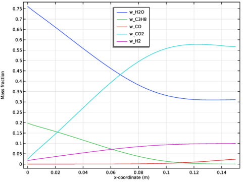
In the Settings window for 1D Plot Group, type Countercurrent Mass Fractions in the Label text field.
|
|
3
|
|
1
|
|
3
|
|
4
|
|
5
|
|
6
|
|
7
|
|
8
|
Clear the Solution checkbox.
|
|
9
|
|
1
|
|
2
|
|
3
|
|
1
|
|
2
|
|
3
|
|
1
|
|
2
|
|
3
|
|
1
|
|
2
|
|
3
|
|
1
|
|
2
|
|
3
|
|
4
|
|
5
|
|
1
|
|
2
|
|
3
|
|
4
|
Click
|
|
1
|
|
2
|
In the Settings window for 3D Plot Group, type Mass fraction, C3H8 Countercurrent in the Label text field.
|
|
3
|
|
4
|
|
5
|
|
6
|
|
1
|
|
2
|
|
3
|
|
4
|
|
1
|
|
2
|
|
3
|
|
4
|
Add the inner wall to the selection by selecting boundary 11 in the Graphics window. Use the scroll wheel to reach interior boundaries.
|
|
1
|
|
2
|
|
1
|
|
2
|
|
3
|
|
4
|
|
1
|
|
3
|
|
4
|
|
1
|
|
2
|
|
3
|
In the Settings window for 3D Plot Group, type Concentration, H2 Countercurrent in the Label text field.
|
|
1
|
|
2
|
In the Settings window for Surface, click Replace Expression in the upper-right corner of the Expression section. From the menu, choose Component 1 (comp1) > Transport of Concentrated Species in Bed > Species w_H2 > tcs.c_w_H2 - Molar concentration - mol/m³.
|
|
3
|
|
1
|
|
2
|
|
3
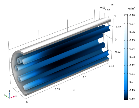
|
In the Settings window for 3D Plot Group, type Gas Density, Countercurrent 900 K in the Label text field.
|
|
1
|
|
2
|
In the Settings window for Surface, click Replace Expression in the upper-right corner of the Expression section. From the menu, choose Component 1 (comp1) > Darcy’s Law in Bed > Material properties > dl.rho - Fluid density - kg/m³.
|
|
3
|
|
4
|
|
1
|
|
2
|
|
3
|
|
4
|
|
5
|
|
6
|
|
1
|
|
2
|
|
3
|
|
4
|
|
1
|
|
2
|
|
3
|
|
1
|
|
2
|
|
1
|
|
1
|
|
2
|
|
3
|
|
4
|
|
1
|
|
2
|
|
3
|
Click
|
|
1
|
|
2
|
|
3
|
|
1
|
In the Settings window for Arrow Surface, click Replace Expression in the upper-right corner of the Expression section. From the menu, choose Component 1 (comp1) > Heat Transfer in Porous Media in Bed > Domain fluxes > ht.tfluxx,...,ht.tfluxz - Total heat flux.
|
|
2
|
|
3
|
|
4
|
|
5
|
|
6
|
|
7
|
|
1
|
|
1
|
|
1
|
|
2
|
In the Settings window for Arrow Surface, click Replace Expression in the upper-right corner of the Expression section. From the menu, choose Component 1 (comp1) > Heat Transfer in Heating Tubes > Domain fluxes > ht2.tfluxx,...,ht2.tfluxz - Total heat flux.
|
|
3
|
|
4
|
|
5
|
|
6
|
|
7
|
Locate the Coloring and Style section.
|
|
8
|
|
9
|
|
10
|
|
1
|
|
2
|
|
3
|
|
4
|
|
5
|
|
6
|
|
1
|
|
2
|
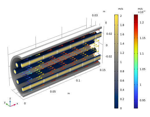
In the Settings window for Volume, click Replace Expression in the upper-right corner of the Expression section. From the menu, choose Default > spf.U - Velocity magnitude - m/s.
|
|
3
|
|
1
|
|
2
|
|
3
|
|
1
|
|
2
|
Click u,v,w - Velocity field in the upper-right corner of the section.
|
|
3
|
|
4
|
|
5
|
|
6
|
|
7
|
|
8
|
|
1
|
|
2
|
|
3
|
|
1
|
In the Settings window for Arrow Volume, click Replace Expression in the upper-right corner of the Expression section. From the menu, choose Component 1 (comp1) > Darcy’s Law in Bed > Velocity and pressure > dl.u,dl.v,dl.w - Total Darcy velocity field.
|
|
2
|
|
1
|
|
2
|
In the Settings window for Color Expression, click Replace Expression in the upper-right corner of the Expression section. From the menu, choose Component 1 (comp1) > Darcy’s Law in Bed > Velocity and pressure > dl.U - Total Darcy velocity magnitude - m/s.
|
|
1
|
|
2
|
|
1
|
|
2
|
|
3
|
|
4
|
|
1
|
|
3
|
|
1
|
|
2
|
|
3
|
Locate the Data section. From the Dataset list, choose Co-current T_in_tubes = 900, 1000 K/Parametric Solutions 1 (sol7).
|
|
1
|
In the Model Builder window, under Results, Ctrl-click to select Countercurrent Mass Fractions, Mass fraction, C3H8 Countercurrent, Concentration, H2 Countercurrent, Gas Density, Countercurrent 900 K, Temperature Countercurrent, and Velocity Countercurrent.
|
|
2
|
Right-click and choose Duplicate.
|
|
1
|
In the Settings window for 1D Plot Group, type Co-current Mass Fractions, 1000 K in the Label text field.
|
|
2
|
Locate the Data section. From the Dataset list, choose Co-current T_in_tubes = 900, 1000 K/Parametric Solutions 1 (sol7).
|
|
3
|
|
4
|
|
5
|
|
1
|
|
2
|
In the Settings window for 3D Plot Group, type Mass fraction, C3H8 Co-current 1000 K in the Label text field.
|
|
3
|
|
4
|
|
1
|
|
2
|
In the Settings window for 3D Plot Group, type Concentration, H2 Co-current 1000 K in the Label text field.
|
|
3
|
|
4
|
|
1
|
|
2
|
In the Settings window for 3D Plot Group, type Gas Density, Co-current 1000 K in the Label text field.
|
|
3
|
|
4
|
|
5
|
|
1
|
|
2
|
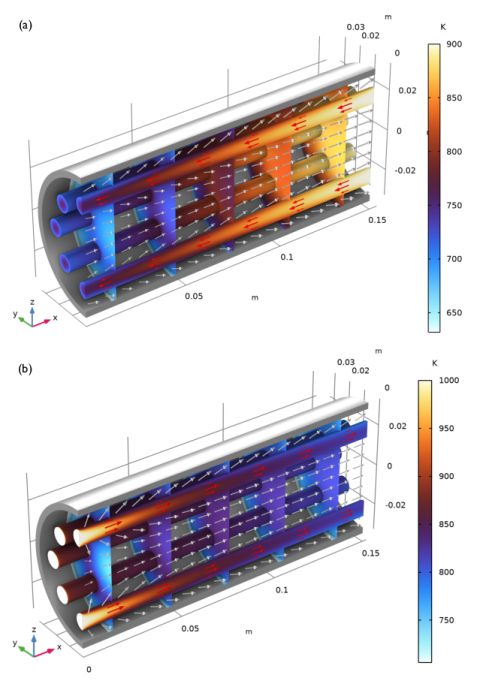
In the Settings window for 3D Plot Group, type Temperature, Co-current 1000 K in the Label text field.
|
|
3
|
|
4
|
|
5
|
|
6
|
|
7
|
|
1
|
|
2
|
|
3
|
|
4
|
|
5
|
|
1
|
In the Model Builder window, under Results, Ctrl-click to select w_C3H8 and T at L/2, Countercurrent Mass Fractions, Mass fraction, C3H8 Countercurrent, Concentration, H2 Countercurrent, Gas Density, Countercurrent 900 K, Temperature Countercurrent, and Velocity Countercurrent.
|
|
2
|
Right-click and choose Group.
|
|
1
|
In the Model Builder window, under Results, Ctrl-click to select Co-current Mass Fractions, 1000 K, Mass fraction, C3H8 Co-current 1000 K, Concentration, H2 Co-current 1000 K, Gas Density, Co-current 1000 K, Temperature, Co-current 1000 K, and Velocity Co-current, 1000 K.
|
|
2
|
Right-click and choose Group.
|
|
1
|
|
2
|
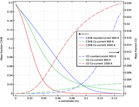
In the Settings window for 1D Plot Group, type w_C3H8 and w_CO Along Bed Midline in the Label text field.
|
|
3
|
|
1
|
|
2
|
|
3
|
Locate the Data section. From the Dataset list, choose Countercurrent T_in_tubes = 900K/Solution 1 (sol1).
|
|
5
|
|
6
|
|
7
|
|
8
|
|
9
|
|
10
|
Clear the Solution checkbox.
|
|
1
|
|
2
|
|
3
|
Locate the Data section. From the Dataset list, choose Co-current T_in_tubes = 900, 1000 K/Parametric Solutions 1 (sol7).
|
|
4
|
|
1
|
|
2
|
|
3
|
|
4
|
|
1
|
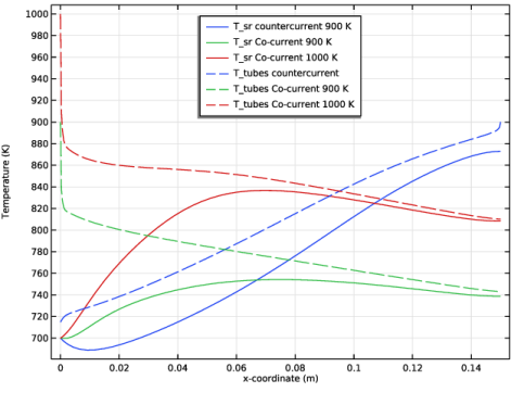
In the Model Builder window, under Results > w_C3H8 and w_CO Along Bed Midline, Ctrl-click to select C3H8 countercurrent 900 K, C3H8 Co-current 900 K, and C3H8 Co-current 1000 K.
|
|
2
|
Right-click and choose Duplicate.
|
|
1
|
|
2
|
|
3
|
Click to expand the Coloring and Style section. Find the Line style subsection. From the Line list, choose Dashed.
|
|
4
|
|
1
|
In the Model Builder window, under Results > w_C3H8 and w_CO Along Bed Midline click C3H8 Co-current 900 K 1.
|
|
2
|
|
3
|
|
4
|
Locate the Coloring and Style section. Find the Line style subsection. From the Line list, choose Dashed.
|
|
1
|
In the Model Builder window, under Results > w_C3H8 and w_CO Along Bed Midline click C3H8 Co-current 1000 K 1.
|
|
2
|
|
3
|
|
4
|
Locate the Coloring and Style section. Find the Line style subsection. From the Line list, choose Dashed.
|
|
1
|
|
2
|
|
3
|
Select the x-axis label checkbox.
|
|
4
|
|
5
|
Select the Two y-axes checkbox.
|
|
6
|
|
7
|
In the table, select the Plot on secondary y-axis checkboxes for CO countercurrent 900 K, CO Co-current 900 K, and CO Co-current 1000 K.
|
|
8
|
|
9
|
|
10
|
|
11
|
|
1
|
|
2
|
In the Settings window for 1D Plot Group, type Temperature Profiles Along Reactor in the Label text field.
|
|
1
|
In the Model Builder window, expand the Temperature Profiles Along Reactor node, then click C3H8 countercurrent 900 K.
|
|
2
|
|
3
|
|
1
|
In the Model Builder window, under Results > Temperature Profiles Along Reactor click C3H8 Co-current 900 K.
|
|
2
|
|
3
|
|
1
|
In the Model Builder window, under Results > Temperature Profiles Along Reactor click C3H8 Co-current 1000 K.
|
|
2
|
|
3
|
|
1
|
In the Model Builder window, under Results > Temperature Profiles Along Reactor click CO countercurrent 900 K.
|
|
2
|
|
3
|
|
5
|
|
1
|
In the Model Builder window, under Results > Temperature Profiles Along Reactor click CO Co-current 900 K.
|
|
2
|
|
3
|
|
5
|
|
1
|
In the Model Builder window, under Results > Temperature Profiles Along Reactor click CO Co-current 1000 K.
|
|
2
|
|
3
|
|
5
|
|
6
|
|
1
|
|
2
|
|
3
|
Clear the Two y-axes checkbox.
|
|
4
|
|
5
|
|
6
|
|
7
|
|
1
|
|
2
|
In the Settings window for Global Evaluation, type Average temperature in bed outflow in the Label text field.
|
|
3
|
Locate the Data section. From the Dataset list, choose Co-current T_in_tubes = 900, 1000 K/Parametric Solutions 1 (sol7).
|
|
4
|
|
5
|
Locate the Expressions section. In the table, enter the following settings:
|
|
6
|
Click
|
|
1
|
|
2
|
In the Settings window for Global Evaluation, type Average temperature in heat tube outflow in the Label text field.
|
|
3
|
Locate the Data section. From the Dataset list, choose Co-current T_in_tubes = 900, 1000 K/Parametric Solutions 1 (sol7).
|
|
4
|
|
5
|
Locate the Expressions section. In the table, enter the following settings:
|
|
6
|
Click
|