|
|
|


|
1
|
|
2
|
|
3
|
Click Add.
|
|
4
|
Click
|
|
5
|
|
6
|
Click
|
|
1
|
|
2
|
|
3
|
Click
|
|
4
|
Browse to the model’s Application Libraries folder and double-click the file lumped_li_battery_parameter_estimation_parameters.txt.
|
|
1
|
In the Model Builder window, under Component 1 (comp1) right-click Definitions and choose Variables.
|
|
2
|
|
3
|
Click
|
|
4
|
Browse to the model’s Application Libraries folder and double-click the file lumped_li_battery_parameter_estimation_variables.txt.
|
|
1
|
|
2
|
|
3
|
|
4
|
|
5
|
Browse to the model’s Application Libraries folder and double-click the file lumped_li_battery_parameter_estimation_E_I_vs_t_data.txt.
|
|
1
|
Go to the Load Cycle Data window.
|
|
1
|
|
2
|
In the Settings window for Interpolation, type Interpolation - E and I vs. t in the Label text field.
|
|
3
|
|
4
|
Locate the Data Column Settings section. In the table, click to select the cell at row number 1 and column number 1.
|
|
5
|
|
7
|
|
9
|
|
1
|
|
2
|
|
3
|
|
4
|
|
5
|
|
1
|
In the Model Builder window, under Component 1 (comp1) > Lumped Battery (lb) click Cell Equilibrium Potential 1.
|
|
2
|
|
3
|
Click
|
|
4
|
Click
|
|
5
|
Browse to the model’s Application Libraries folder and double-click the file lumped_li_battery_parameter_estimation_E_OCP_data.txt.
|
|
6
|
|
1
|
|
2
|
|
3
|
Select the Include concentration overpotential checkbox.
|
|
1
|
|
2
|
|
1
|
|
2
|
|
3
|
|
4
|
|
5
|
|
6
|
|
1
|
|
2
|
|
3
|
|
4
|
|
1
|
|
2
|
|
1
|
|
2
|
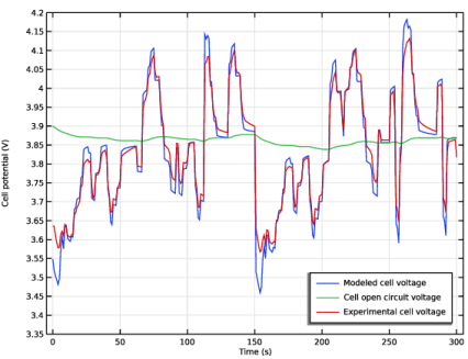
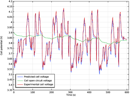
In the Settings window for Global, click Replace Expression in the upper-right corner of the y-Axis Data section. From the menu, choose Component 1 (comp1) > Definitions > Variables > E_cell_exp - Experimental cell voltage - V.
|
|
1
|
|
2
|
|
3
|
Select the Manual axis limits checkbox.
|
|
4
|
|
5
|
|
6
|
|
7
|
|
1
|
|
1
|
|
2
|
|
1
|
|
2
|
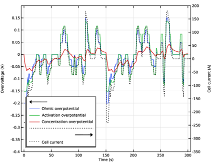
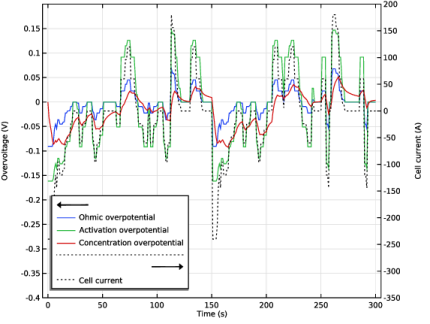
In the Settings window for Global, click Replace Expression in the upper-right corner of the y-Axis Data section. From the menu, choose Component 1 (comp1) > Lumped Battery > Overpotentials > lb.eta_ir - Ohmic overpotential - V.
|
|
3
|
Click Add Expression in the upper-right corner of the y-Axis Data section. From the menu, choose Component 1 (comp1) > Lumped Battery > Overpotentials > lb.eta_act - Activation overpotential - V.
|
|
4
|
Click Add Expression in the upper-right corner of the y-Axis Data section. From the menu, choose Component 1 (comp1) > Lumped Battery > Overpotentials > lb.eta_conc - Concentration overpotential - V.
|
|
5
|
|
6
|
|
1
|
|
2
|
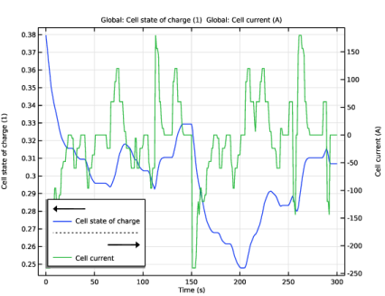
In the Settings window for Global, click Replace Expression in the upper-right corner of the y-Axis Data section. From the menu, choose Component 1 (comp1) > Lumped Battery > lb.I_cell - Cell current - A.
|
|
3
|
|
4
|
|
5
|
Click to expand the Coloring and Style section. Find the Line style subsection. From the Line list, choose Dotted.
|
|
6
|
|
1
|
|
2
|
|
3
|
|
4
|
Locate the Plot Settings section.
|
|
5
|
|
6
|
Select the Two y-axes checkbox.
|
|
7
|
|
8
|
|
9
|
|
10
|
|
11
|
|
12
|
|
13
|
|
14
|
|
15
|
|
1
|
In the Model Builder window, under Component 1 (comp1) > Lumped Battery (lb) click Voltage Losses 1.
|
|
2
|
|
3
|
|
4
|
|
5
|
|
6
|
|
1
|
|
2
|
Go to the Add Study window.
|
|
3
|
|
4
|
Click the Add Study button in the window toolbar.
|
|
5
|
|
1
|
|
2
|
|
1
|
|
2
|
|
3
|
|
4
|
Locate the Data Column Settings section. In the table, enter the following settings:
|
|
6
|
|
7
|
|
8
|
|
10
|
Locate the Parameter Estimation Method section. Find the Solver settings subsection. From the Least-squares time/parameter list method list, choose Use only least-squares data points.
|
|
1
|
In the Model Builder window, under Component 1 (comp1) right-click Definitions and choose Global Variable Probe.
|
|
2
|
|
3
|
|
1
|
|
2
|
|
3
|
|
1
|
|
2
|
|
3
|
|
1
|
|
1
|
|
2
|
|
3
|
|
4
|
|
1
|
|
2
|
|
3
|
|
4
|
|
1
|
|
2
|
|
3
|
Select the Plot checkbox.
|
|
1
|
|
2
|
|
3
|
|
4
|
Browse to the model’s Application Libraries folder and double-click the file lumped_li_battery_parameter_estimation_E_I_vs_t_fulldata.txt.
|
|
1
|
Go to the Full Load Cycle Data window.
|
|
1
|
|
2
|
In the Settings window for Interpolation, type Interpolation - E and I vs. t (full) in the Label text field.
|
|
3
|
|
4
|
|
5
|
Locate the Data Column Settings section. In the table, click to select the cell at row number 1 and column number 1.
|
|
6
|
|
8
|
|
10
|
|
1
|
In the Model Builder window, under Component 1 (comp1) > Definitions right-click Variables 1 and choose Duplicate.
|
|
2
|
|
1
|
|
2
|
Go to the Add Study window.
|
|
3
|
|
4
|
Click the Add Study button in the window toolbar.
|
|
5
|
|
1
|
In the Model Builder window, under Study 3 - Full Load Curve Prediction click Step 1: Time Dependent.
|
|
2
|
|
3
|
|
4
|
|
5
|
|
6
|
Locate the Physics and Variables Selection section. Select the Modify model configuration for study step checkbox.
|
|
7
|
|
8
|
Click
|
|
9
|
Click to expand the Values of Dependent Variables section. Find the Initial values of variables solved for subsection. From the Settings list, choose User controlled.
|
|
10
|
Find the Values of variables not solved for subsection. From the Settings list, choose User controlled.
|
|
11
|
|
12
|
|
13
|
|
14
|
|
15
|
Clear the Generate default plots checkbox.
|
|
1
|
|
2
|
|
3
|
Select the Modify model configuration for study step checkbox.
|
|
4
|
|
5
|
Click
|
|
1
|
|
2
|
|
3
|
Select the Modify model configuration for study step checkbox.
|
|
4
|
|
5
|
Click
|
|
1
|
|
2
|
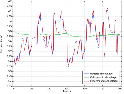
In the Settings window for 1D Plot Group, type Cell Voltage: Full Cycle Prediction in the Label text field.
|
|
3
|
Locate the Data section. From the Dataset list, choose Study 3 - Full Load Curve Prediction/Solution 3 (sol3).
|
|
4
|
|
5
|
|
1
|
In the Model Builder window, expand the Cell Voltage: Full Cycle Prediction node, then click Global 1.
|
|
2
|
|
4
|
|
1
|
|
2
|
In the Settings window for Global Evaluation, type Global Evaluation: Standard Deviation (Study1) in the Label text field.
|
|
3
|
Locate the Expressions section. In the table, enter the following settings:
|
|
4
|
|
5
|
Click
|
|
1
|
|
2
|
In the Settings window for Global Evaluation, type Global Evaluation: Standard Deviation (Study2) in the Label text field.
|
|
3
|
Locate the Data section. From the Dataset list, choose Study 2 - Parameter Estimation/Solution 2 (sol2).
|
|
4
|
Click
|
|
1
|
|
2
|
In the Settings window for Global Evaluation, type Global Evaluation: Standard Deviation (Study3) in the Label text field.
|
|
3
|
Locate the Data section. From the Dataset list, choose Study 3 - Full Load Curve Prediction/Solution 3 (sol3).
|
|
4
|
|
5
|
|
6
|
Click
|