
|
|
|
|
5.997·107 S/m
|
|||
|
103-10i
|
|
1
|
|
2
|
In the Select Physics tree, select AC/DC > Electromagnetic Fields > Vector Formulations > Magnetic and Electric Fields (mef).
|
|
3
|
Click Add.
|
|
4
|
Click
|
|
5
|
|
6
|
Click
|
|
1
|
|
2
|
|
3
|
Click
|
|
4
|
Browse to the model’s Application Libraries folder and double-click the file power_inductor.mphbin.
|
|
5
|
Click
|
|
1
|
|
2
|
|
3
|
|
4
|
|
5
|
|
6
|
|
7
|
|
8
|
|
9
|
Click
|
|
10
|
|
1
|
|
2
|
Go to the Add Material window.
|
|
3
|
|
4
|
Click the Add to Component button in the window toolbar.
|
|
5
|
|
1
|
|
2
|
Click
|
|
1
|
|
2
|
In the Settings window for Magnetic and Electric Fields, click to expand the Discretization section.
|
|
3
|
|
4
|
|
1
|
|
1
|
|
3
|
|
4
|
|
1
|
|
1
|
|
3
|
In the Settings window for Ampère’s Law and Current Conservation in Solids, locate the Constitutive Relation B-H section.
|
|
4
|
|
1
|
In the Model Builder window, under Component 1 (comp1) right-click Materials and choose Blank Material.
|
|
2
|
|
4
|
Locate the Material Contents section. In the table, enter the following settings:
|
|
1
|
|
2
|
|
3
|
|
4
|
|
5
|
|
1
|
|
2
|
|
3
|
|
5
|
|
6
|
Locate the Element Size Parameters section.
|
|
7
|
|
1
|
|
2
|
|
3
|
|
1
|
|
3
|
|
4
|
|
5
|
|
6
|
|
7
|
Click
|
|
1
|
|
2
|
|
3
|
|
4
|
Locate the Physics and Variables Selection section. Select the Modify model configuration for study step checkbox.
|
|
5
|
In the tree, select Component 1 (comp1) > Magnetic and Electric Fields (mef) > Gauge Fixing for A-field 1.
|
|
6
|
Right-click and choose Disable.
|
|
1
|
|
2
|
|
3
|
In the Model Builder window, expand the Study 1 > Solver Configurations > Solution 1 (sol1) > Stationary Solver 1 node, then click Iterative 1.
|
|
4
|
|
5
|
|
6
|
|
7
|
|
8
|
|
9
|
Right-click Study 1 > Solver Configurations > Solution 1 (sol1) > Stationary Solver 1 > Iterative 1 and choose SOR.
|
|
10
|
|
11
|
Clear the Generate default plots checkbox.
|
|
12
|
|
13
|
|
1
|
|
2
|
Go to the Add Study window.
|
|
3
|
|
4
|
Click the Add Study button in the window toolbar.
|
|
5
|
|
1
|
|
2
|
|
1
|
|
2
|
|
3
|
In the Model Builder window, expand the Study 2 > Solver Configurations > Solution 2 (sol2) > Stationary Solver 1 node, then click Fully Coupled 1.
|
|
4
|
|
5
|
|
6
|
|
7
|
|
8
|
|
9
|
|
1
|
|
2
|
|
3
|
|
5
|
Click
|
|
1
|
Go to the Table 1 window.
|
|
1
|
|
3
|
|
5
|
|
1
|
|
2
|
|
3
|
|
4
|
|
1
|
Go to the Table 1 window.
|
|
2
|
|
1
|
|
2
|
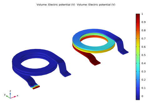
In the Settings window for 3D Plot Group, type Electric Potential, Comparison in the Label text field.
|
|
3
|
|
1
|
|
2
|
|
3
|
|
1
|
|
1
|
In the Model Builder window, under Results > Electric Potential, Comparison right-click Volume 1 and choose Duplicate.
|
|
2
|
|
3
|
|
4
|
|
1
|
|
2
|
|
3
|
|
4
|
|
5
|
|
6
|
|
1
|
|
2
|
|
3
|
|
1
|
|
2
|
|
3
|
|
1
|
|
2
|
|
3
|
|
4
|
|
1
|
|
2
|
In the Settings window for 3D Plot Group, type Electric Potential, Gauged Formulation in the Label text field.
|
|
3
|
|
1
|
|
2
|
Select Boundaries 3 and 5–79 only. The quickest way to do this is to select All boundaries from the Selection list, then remove Boundaries 1, 2, and 4.
|
|
1
|
|
2
|
|
3
|
Click
|